JASP for beginners
Ihnwhi Heo, Duco Veen, and Rens van de Schoot
Department of Methodology and Statistics, Utrecht University
Last modified: 31 August 2020
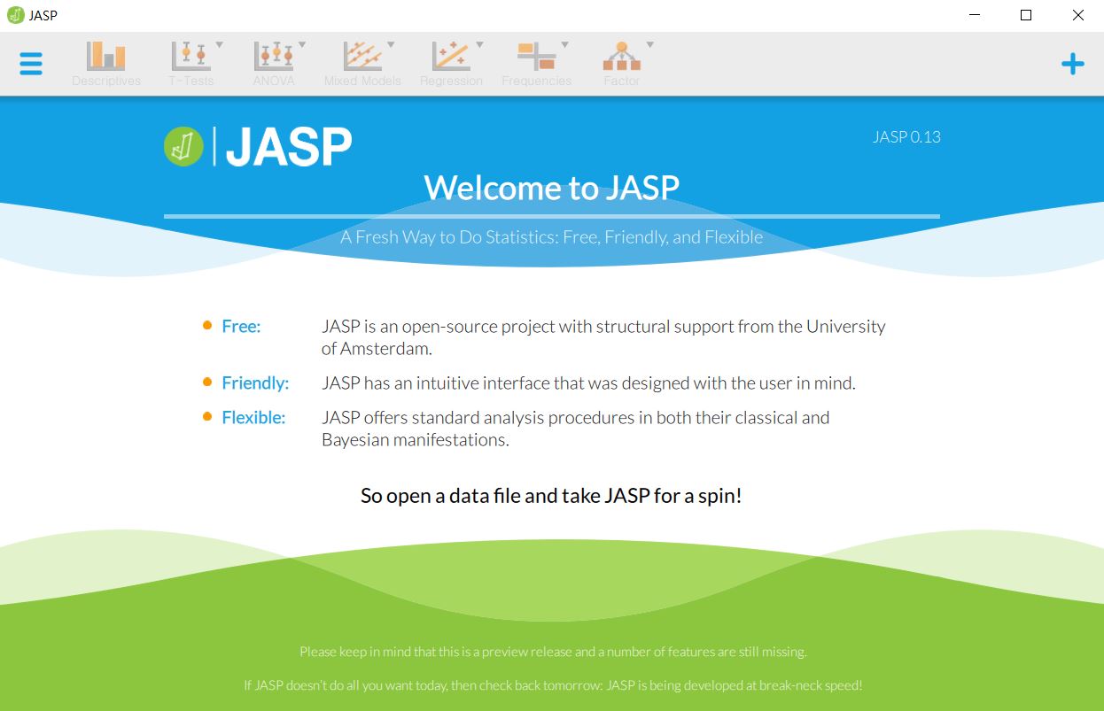
Welcome to the world of JASP!
This tutorial introduces the fundamentals of JASP (JASP Team, 2020) for starters. Our explanation starts with the installation of JASP, the screen structure of JASP, and loading data.
Given the data loaded, we explore data via descriptive statistics and data visualization. We further explain how to perform correlation analysis, multiple linear regression, t-test, and one-way analysis of variance from a frequentist perspective and draw conclusions from outputs.
Since we continuously improve the tutorials, let us know if you discover mistakes, or if you have additional resources we can refer to. If you want to be the first to be informed about updates, follow Rens on Twitter.
Let’s get started!
How to cite this tutorial in APA style
Heo, I., Veen, D., & Van de Schoot, R. (2020, July). Tutorial: JASP for beginners. Zenodo. https://doi.org/10.5281/zenodo.4008280
Popularity Dataset
We will use a popularity dataset (Van de Schoot, 2020) from Van de Schoot, Van der Velden, Boom, and Brugman (2010). To download the dataset, click here.
The dataset is based on a study that investigates an association between popularity status and antisocial behavior from at-risk adolescents (n = 1491), where gender and ethnic background are moderators under the association. The study distinguished subgroups within the popular status group in terms of overt and covert antisocial behavior.
For more information on the sample, instruments, methodology, and research context, we refer the interested readers to the paper (see references). A brief description of the variables in the dataset follows. The variable names in the table below will be used in the tutorial, henceforth.
| Variable name | Description |
|---|---|
| respnr | Respondents’ number |
| Dutch | Respondents’ ethnic background (0 = Dutch origin, 1 = non-Dutch origin) |
| gender | Respondents’ gender (0 = boys, 1 = girls) |
| sd | Adolescents’ socially desirable answering patterns |
| covert | Covert antisocial behavior |
| overt | Overt antisocial behavior |
How to cite the dataset in APA style
Van de Schoot, R. (2020). Popularity Dataset for Online Stats Training [Data set]. Zenodo. https://doi.org/10.5281/zenodo.3962123
I. What is this thing called JASP?
1. A rising star in statistical software
- Free and open-source software for statistical analysis
- Easy, intuitive, and simple to use
- Extensive: available from basic (e.g., t-test, regression, ANOVA) to advanced analytic techniques (e.g., machine learning, structural equation modeling, meta-analysis, network analysis)
- Inclusive: geared for both frequentist and Bayesian statistics
- Many resources by the JASP team
- Comparison between JASP and SPSS

(Image source: Jonas Kristoffer Lindeløv at Aalborg University)
2. Invite JASP to your PC: Installation
- Click here to start downloading.
- Consider your operating system (Windows, Mac, Linux).
- If you use Windows, click
JASP for Windows. - If you use Mac, click
JASP for Mac.- Problems in installing under Mac? Click here.
- If you use Windows, click
- If you use Linux, click
Linux Installation Guide-> Open the terminal -> Run the installation command. - If you want to download a previous version rather than the latest version, click here.
3. Eye contact with JASP
- Let’s open the JASP. What is your first impression of JASP?
- JASP has a simple screen structure. When you load any data (not explained yet, but you will see!), you can proceed with everything from three sections.
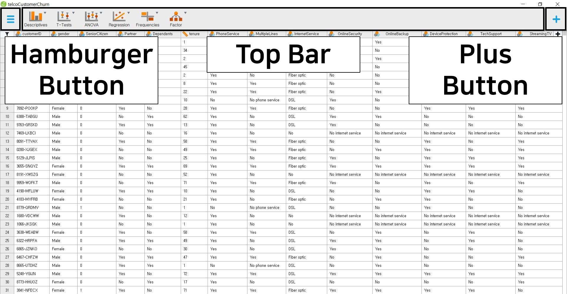
- Let us give you a brief explanation of the three parts on the screen.
Hamburger button (top left)

- What we mean by the hamburger button is not the real hamburger (unfortunately!) but the abstract hamburger-like button with three layers.
- To eat the ‘hamburger’, the only thing you have to do is a simple mouse click.
- With the hamburger button, you can open, save, or export data.
Top bar (top middle)

- As you might have guessed, the top bar is a group of primary analyses. You can simply start any analysis you want by clicking the analysis option. For example, if you want to perform regression analysis, simply click the ‘Regression’ button. Do you want to know the next step? We will guide you through the steps in ‘IV. Data analysis and interpretation’. So please follow our guidance until that section.
- “Wait, are the six options all things I can do?” Not at all! You can run more advanced statistical analyses. How? Let’s look at the plus button below.
Plus button (top right)

- As the ‘plus’ sign implies, the plus button is an add-on button for advanced analytic techniques.
- When you click the plus button, you can encounter various analysis options such as JAGS, Machine Learning, Meta-Analysis, Network, SEM (Structural Equation Modeling), and more. They will help you answer the complex research questions.
- Let’s imagine you want to implement the structural equation modeling in JASP. To do that, you need to add the SEM option in the top bar.
- Click the plus button and check the square box located at the left of the word ‘SEM’. You can immediately notice the SEM option is added to the top bar.

- You can remove the SEM option from the top bar. Click the plus button again and uncheck the square box. Can you see the SEM option has disappeared from the top bar? Great!
II. Provide JASP with data
- We proceed statistical analyses with data. You can simply load the data with several mouse clicks. From where? Yes, the hamburger button!
- JASP offers data loading not only from your computer but also from the in-built data library or the Open Science Framework.
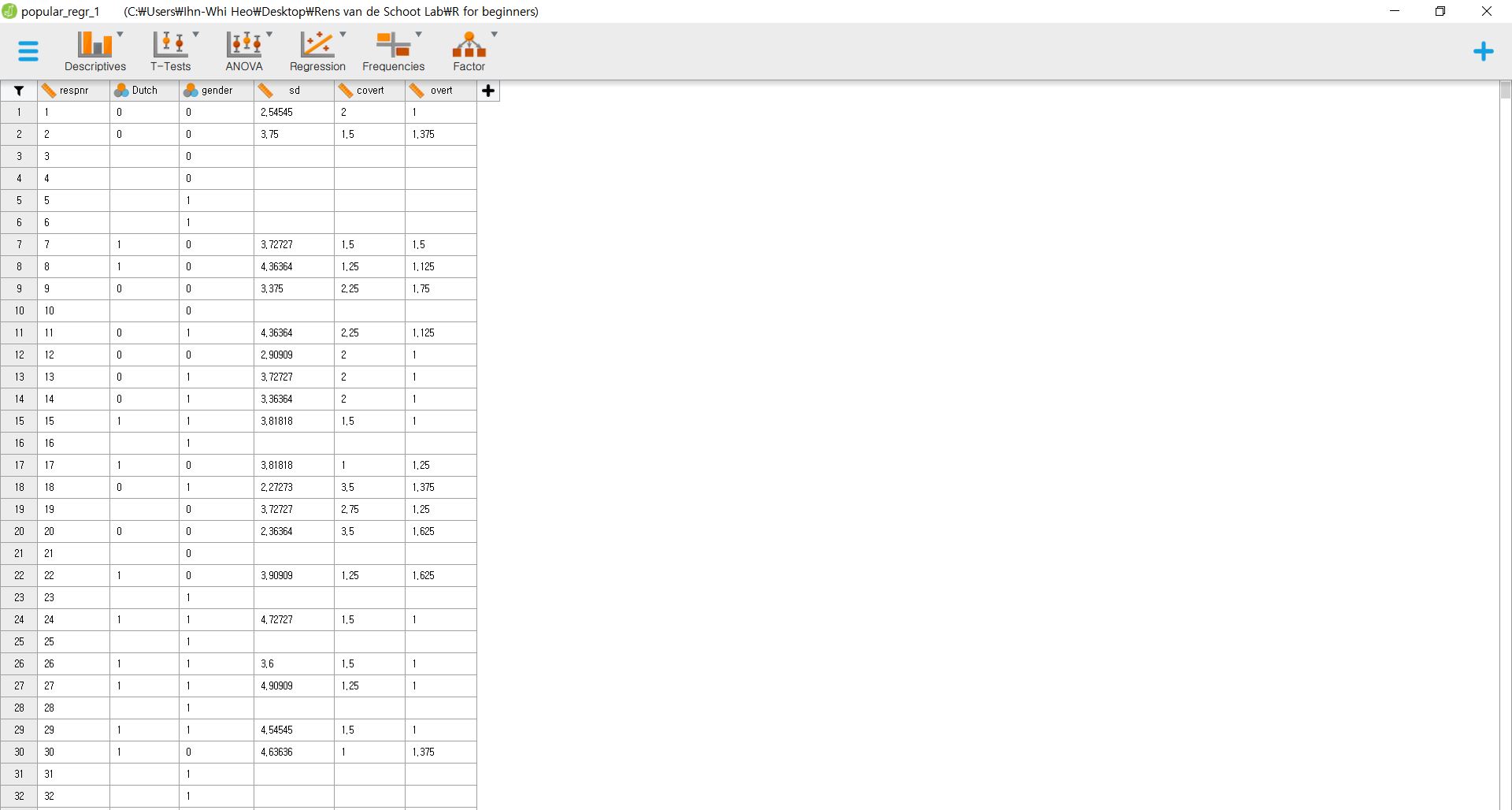
- To download the dataset that we will use (
popular_regr_1), click here.
1. From your computer
- Click hamburger button -> Open -> Computer -> Browse -> Open your file

- That is all you should do. How simple! Do you see the loaded dataset or the spreadsheet as the below picture?
- There is one tip after you load the data. Let’s imagine you are scrolling up and down to check whether the JASP correctly loaded the data and whether all entries are correct. Suddenly, you detected that some data entries are wrong, so you need to fix some values. Do we have to close the JASP, open the data file, fix the errors, and load the data on JASP again? Fortunately, we do not need to!
- If you double click the loaded dataset or spreadsheet on the JASP screen, the JASP automatically links to the original data file (in our case, the SPSS file). What you need to do, then, is to change the values, save and close the SPSS file. Since the JASP synchronizes with the data file, you can see that what you have changed is already reflected in JASP. In this way, you can work efficiently.
- Now, we are ready to explore and analyze the data. For didactic purposes, we also provide how to load the data from the in-built data library or the Open Science Framework. You can skip the below explanation and go to ‘III. Data exploration’ or ‘IV. Data analysis and interpretation’ if you cannot wait to see how easily you can explore and analyze the data with JASP!
2. From the data library
- JASP provides in-built datasets that are relevant for the specific type of analyses that one would like to perform. Let’s imagine again that we want to perform the structural equation modeling (SEM), so we need to load the dataset for the SEM.
- Click hamburger button -> Open -> Data Library -> Choose the statistical analysis you want to perform -> Click SEM (Of course, you can choose other analyses depending on your needs) -> Click Political Democracy
3. From the OSF projects
- What is the Open Science Framework (henceforth OSF)? To simply put, the OSF is a free and open platform that researchers can share their projects and data. For interested readers, we recommend the two websites that illustrate the OSF.
- To load the data from your OSF, you have to log in to your OSF account and there should be a dataset in your OSF project. If you have your data uploaded on the OSF website, you can load directly from the project without downloading it to the computer.
- Click hamburger button -> Open -> OSF -> Sign in with your OSF account -> Choose your project -> Open your file

III. Data exploration
1. Understanding the data with numbers
Descriptive statistics
- Do you want to know the mean, the median, the maximum value, and more about the variables in your data? What you need to look at is the descriptive statistics. Let’s investigate the descriptive statistics of the variables in the
popular_regr_1dataset. - Go to the top bar -> Click Descriptives -> Descriptive Statistics -> Move the six variables to the ‘Variables’ section on the right. How? Click the right-headed triangle button after selecting the six variables
- “What are the symbols with the variable names?” Good observation! They indicate the measurement level of the corresponding variables. For example, a symbol that looks like a ruler means a scale variable (also called a continuous variable). A symbol with three colorful circles refers to a nominal variable. Readers who use SPSS can see that those symbols are identical to those in the SPSS.
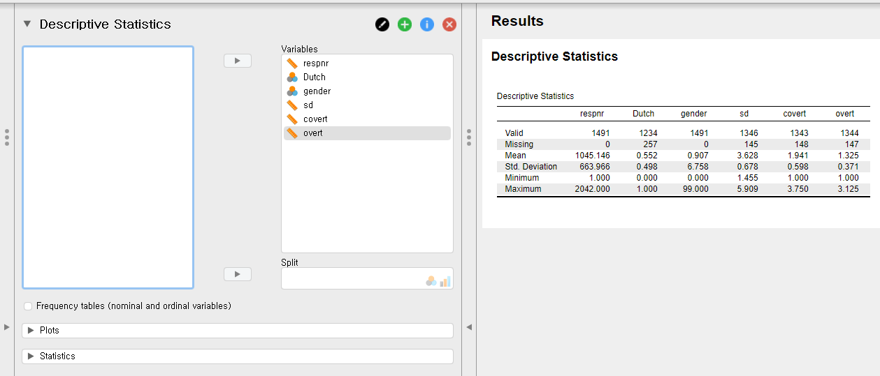
- Right after you move the variables, JASP immediately prints the output on the right section of the screen.
- For convenience, let us refer to a left panel as a control panel and a right panel as an output panel.
- Look at the output panel (right panel). You can see the table with descriptive statistics. In the first column of the table, there are six rows. Valid shows sample size after excluding the missing values. For the variable overt, there are 1344 ‘valid’ entries. The number of missing values, in contrast, is at the Missing row. For overt, there are 147 missing values. Consequently, the sum between Valid and Missing is the total sample size for each variable. For overt, there are 1491 samples, which equals 1344 plus 147. The mean and the standard deviation (Mean and Std. Deviation in the first column) of overt are 1.325 and 0.371. The maximum and minimum value (Maximum and Minimum in the first column) are 1 and 3.125.
- What if we want to investigate more descriptive statistics, such as the median, the mode, the range, the skewness, and so forth? Look at the control panel (left panel). What you need to conduct is to click the Statistics bar at the bottom left of the control panel and check Median and Mode under Central Tendency, Range under Dispersion, and Skewness under Distribution.
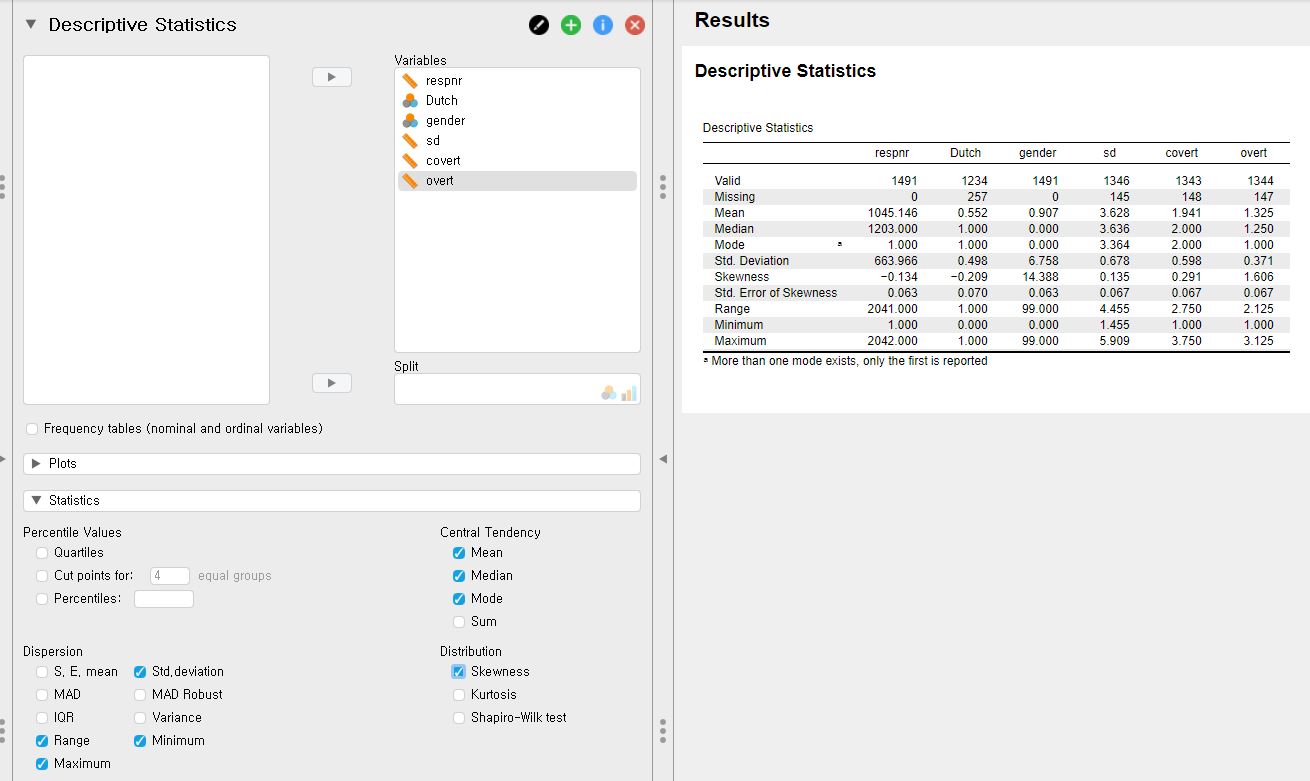
- JASP again gives the descriptive statistics you selected immediately on the output panel. For example, the median and the range of overt are 1.250 and 2.125.
Frequency tables
- In case there are categorical variables (nominal and ordinal variables), frequency tables show the frequency of each category (a category is also called as a level in statistics).
- Check Frequency tables (nominal and ordinal variables) in the control panel. The checkbox of Frequency tables is roughly located in the middle of the control panel.
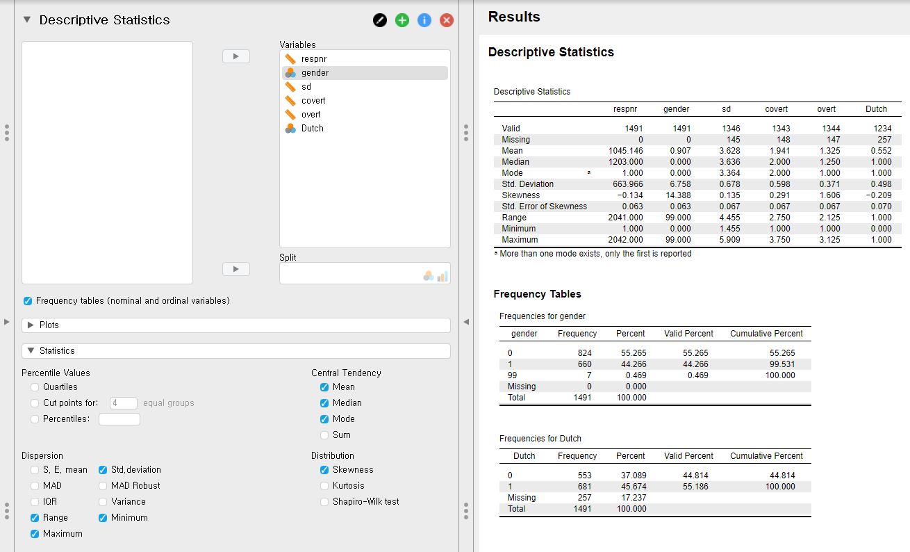
- Since there are two categorical variables, gender and Dutch, two frequency tables are created. For example, let’s look at the frequency table for Dutch.
- There are 553 cases coded as 0 and 681 coded as 1. Also, there are 257 missing values. The missing value consists of about 17.24% of the total samples of the Dutch variable.
2. Getting insight from the visual inspection
- In the world of statistics, images usually speak louder than words. Think about the skewness of the variable we examined before. Rather than a number, looking at the distribution is more intuitive.
- With some simple mouse clicks, JASP provides information about the data with neat plots.
- Let’s start from the place where we ended. That is, we will start plotting from putting all six variables under the Variables section.
Distribution plots
- If you want to visually inspect the distribution of your data of certain variables, making distribution plots is the one you should perform.
- Click Plots bar in the control panel -> Check Distribution plots under Basic plots
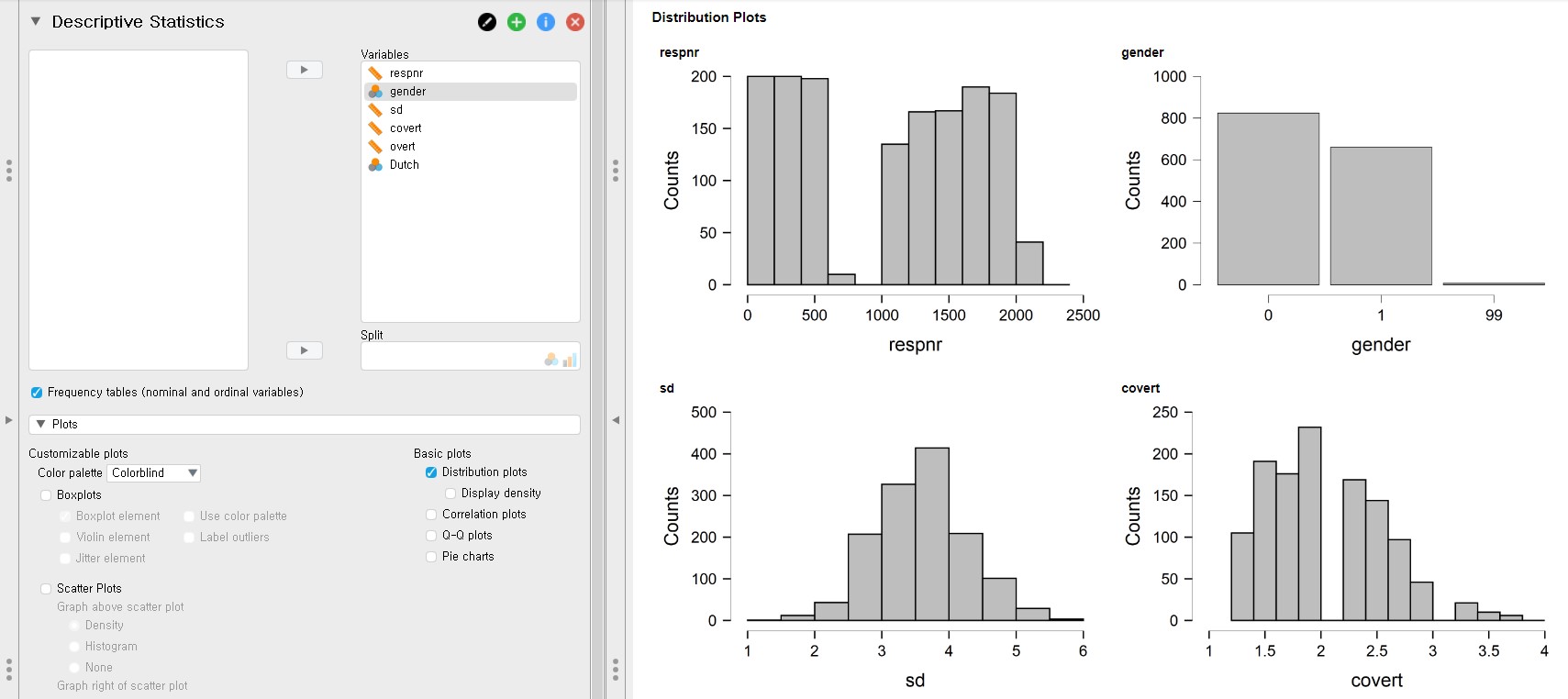
- JASP produces histograms for scale variables and frequency plots for categorical variables. Variable names are indicated on top of the y-axis.
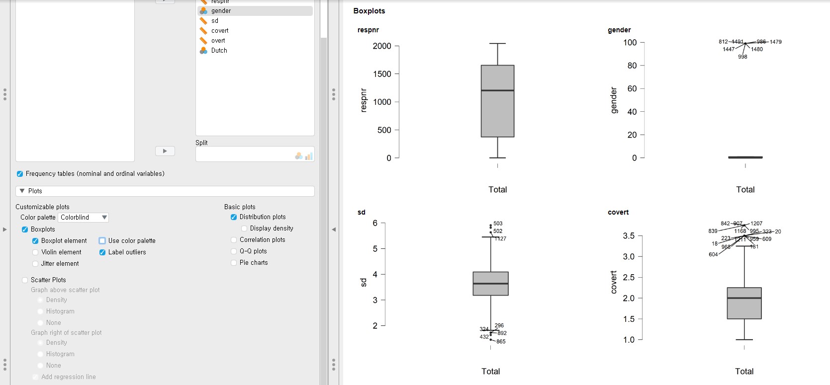
Boxplots
- Boxplot is a good way of investigating the dispersion of the data from the median and checking the existence of outliers.
- Click Plots bar in the console panel -> Check Boxplots -> Check Boxplot element under Boxplots
- Depending on your needs, you can add additional features in the boxplot, for example, checking Label outliers indicates which case of the variable is an outlier.
Scatter plots
- Scatter plots are wise decisions when you want to describe the relationship between two variables.
- Click Plots bar on the control panel -> Check Scatter Plots -> Depending on your needs, you can add additional features in the scatter plots.
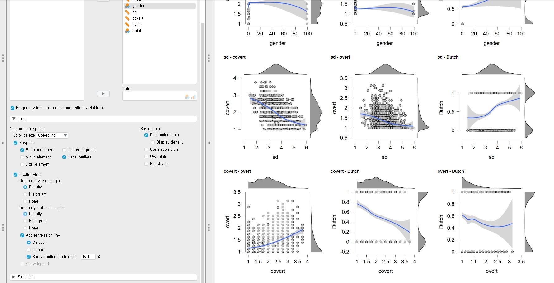
- You must be surprised or intimidated at the plots that JASP prints. Don’t be scared! There are all scatter plots but with additional features to understand the relationship between two variables more in-depth. The dots are the actual data points. Graphs above the scatter plots are density (or distribution in a more intuitive term) of the variable at the x-axis. Graphs right of the scatter plots are a density of the variable at the y-axis. Blue lines are regression lines but in a smoothed (or curved in a more intuitive term) way. The grey-shaded area around the regression lines is 95% confidence intervals.
- You can change the type of graphs above or right of the scatter plots. It is also possible to change the smoothed regression lines to the linear ones and remove the confidence intervals. All you need to do is to click the various settings under Scatter Plots in the control panel.
IV. Data analysis and interpretation
- In this tutorial, we fully focus on basic statistical analysis in the frequentist statistics framework. However, it does not mean we will never deal with Bayesian stuff. After this introductory JASP tutorial, you can study another tutorial that explains how to perform Bayesian statistics in JASP.
- At this point, readers might be curious about what exactly the Bayesian statistics is, what the differences are compared to frequentist statistics, and how it helps substantive research. For interested readers, we refer to two great easily-written papers with the links!
- A gentle introduction to Bayesian analysis: Applications to developmental research (Van de Schoot, Kaplan, Denissen, Asendorpf, Neyer, & Van Aken, 2014)
- Bayesian analyses: Where to start and what to report (Van de Schoot & Depaoli, 2014)
- We assume that all the assumptions required for subsequent analyses are satisfied.
1. Correlation analysis
- If you want to test whether the correlation coefficient between two variables is significantly different from 0, you have to conduct correlation analysis.
- Go to the top bar -> Click Regression -> Correlation under Classical section -> Choose at least two variables
- Let’s run the correlation analysis to investigate whether the correlation coefficient between the covert and overt antisocial behavior (covert and overt) is significantly different from 0.
- From now on, we will use the alpha level of .05 because it is most commonly used.
- To do so, move the two variables, overt and covert, under the Variables section.
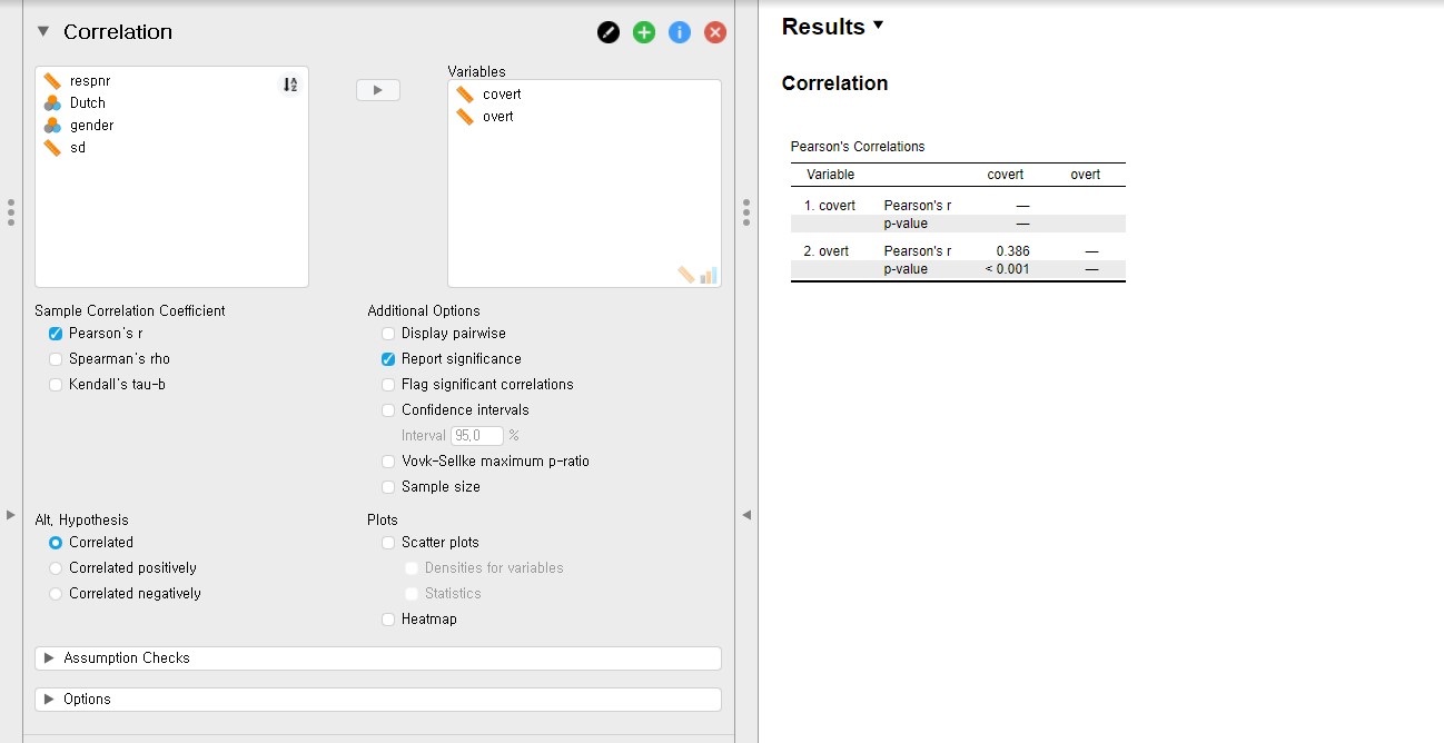
- The correlation coefficient between covert and overt is 0.386 and the p-value is lower than 0.001, according to the output in the output panel. Therefore, the correlation coefficient of 0.386 is significantly different from 0.
2. Multiple linear regression
- Multiple linear regression analysis is performed when you are interested in predicting outcomes of a continuous dependent variable with multiple continuous or categorical independent variables.
- Go to the top bar -> Click Regression -> Click Linear Regression under Classical section -> Choose one variable for Dependent Variable and other variables for Covariates (Covariates refer to independent variables)
- For illustrative purposes, let’s try to predict adolescents’ socially desirable answering patterns (sd) with overt and covert antisocial behavior (overt and covert). Consequently, we have to use sd as the dependent variable and overt and covert as the independent variables. Move sd under the Dependent Variable section and covert and overt under the Covariates section.
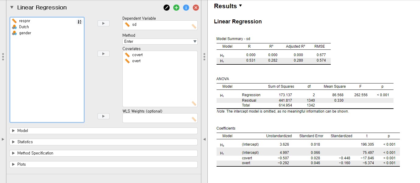
- First, look at the table under Coefficients in the output panel.
- The unstandardized regression coefficient of covert is -0.507, and the p-value is lower than 0.001. You can find this value at the cross-section between the covert row of H1 and the Unstandardized column. This result means that the variable, covert, is a significant predictor with an alpha level of .05. If one unit of covert increases, the sd decreases 0.507 units.
- The unstandardized regression coefficient of overt is -0.292 with the p-value lower than 0.001. Therefore, the variable, overt, is a significant predictor of sd with an alpha level of .05. If one unit of overt increases, the sd decreases 0.292 units.
- The standardized regression coefficients can be found under the Standardized column. The standardized regression coefficients are used to compare the effect sizes among predictors. These coefficients are scaled to one standard deviation. Therefore, if one standard deviation of covert increases, 0.448 standard deviations of sd decreases. On the other hand, if one standard deviation of overt increases, 0.160 standard deviations of sd decreases. Therefore, the strength of covert in predicting sd is greater than that of overt.
- Second, let’s look at the R-squared, which is indicated in the table under Model Summary. You have to look at the H1 row. The R-squared is the proportion of variance explained by predictors. Therefore, the R-squared value of 0.280 means that the two predictors, covert and overt, explain 28% of the variance of sd.
- Last, let’s look at the F-statistic in the table under ANOVA. The F-statistic in the regression model indicates whether the model fits the data well. Let’s see the p-value of the F-statistic. Because the p-value of the F-statistic is lower than 0.001, the regression model fits significantly better than the model that does not contain any predictors.
3. t-test
- A t-test is an option when you are keen on examining whether the means of certain variables between the two groups significantly differ from each other.
- Go to the top bar -> Click T-Tests -> Click Independent Samples T-Test under Classical section
- Among variables in our dataset, let’s test whether the means of covert antisocial behavior (covert) between the respondents’ different ethnic backgrounds (Dutch) are significantly different.
- Move the covert variable under the Variables section and the Dutch variable under the Grouping Variable section.
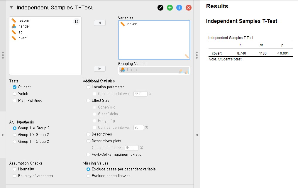
- The p-value is lower than 0.001. Thus, the two means of covert between two groups of the Dutch variable are significantly different from each other.
4. One-way analysis of variance
- If you are interested in examining whether the means are significantly different across groups, one-way analysis of variance answers your question.
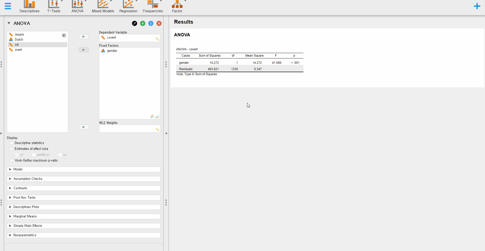
- Go to the top bar -> Click ANOVA -> Click ANOVA under Classical section -> Choose one dependent variable for Dependent Variable and grouping variables for Fixed Factors
- Let’s examine whether the means of the covert antisocial behavior (covert) are significantly different across respondents’ genders (gender).
- Before proceeding further, there is one thing we should do. According to the frequency table of gender in ‘III. Data exploration’, the gender variable has three categories: 0, 1, and 99. Since JASP treats 99 as an independent category, which is not the case, it is necessary to filter 99 out.
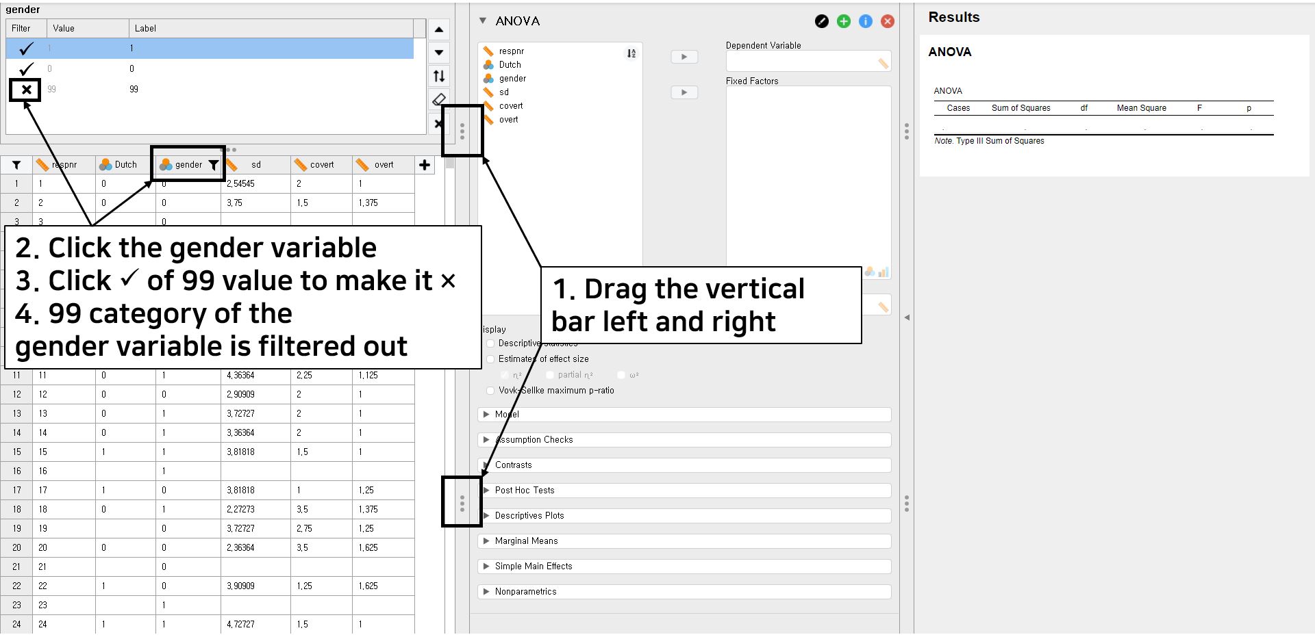
- One tip to simultaneously look at the spreadsheet, the control panel, and the output panel is to horizontally drag the tab with three vertical dots.
- Click the gender variable of the spreadsheet. We will now try to filter the 99 value of the gender variable out.
- Simply click the check sign at the left of the 99 value. You can see that the X sign appears instead of the check sign. In this way, we filter the 99 value out.
- It is fine to go! Move the covert variable under the Dependent Variable section and the gender variable under the Fixed Factors section.
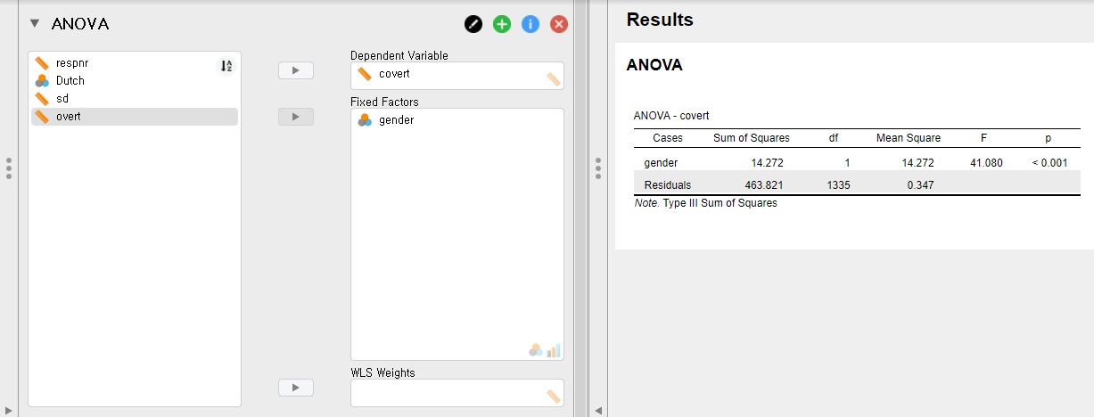
- The p-value of gender is lower than 0.001. Therefore, there are significant mean differences in covert between the two genders.
5. Additional tips that will make you a smart JASP user
Playing with the output panel
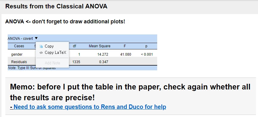
- The above picture shows everything we would like to tell you.
- In the output panel, you can edit the title or add notes so that your process, questions, or anything noticeable can be written. This will help you when you need to return to the outputs later. Also, your collaborators can follow the updates.
- One helpful functionality is to copy the table or extract the LaTeX code by right-clicking the mouse at the table. Copying the LaTeX code is especially useful since it saves your time a lot when you do documentation with LaTeX. Furthermore, the code contributes to the reproducibility of your results!
Exporting your result to OSF projects
- Do you remember that we can import the data from the OSF? It is also possible to export the data or the results from the JASP to OSF directly. Here, we emphasize the usefulness and importance of exporting the results to the OSF projects.
- To export the results, follow this step: Click Hamburger button -> Export Results -> OSF -> Choose the corresponding project -> Choose the place you want to export the result
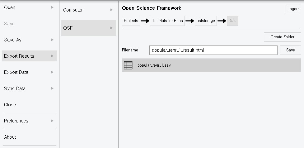
- Our results are exported to the OSF projects as an HTML format. Exporting the figures or tables from the output is helpful for the final check or publication purposes.
V. Epilogue
- Congratulations! You have finished all the basic but core practices to use the JASP. We hope you enjoyed this tutorial.
- We are going to end this tutorial with two additional points. Take it easy and enjoy the ending!
1. The greatest synergy between JASP and Bayesian statistics
- As mentioned at the beginning of ‘IV. Data analysis and interpretation’, we only focused on statistical analyses from the frequentist statistics perspective. One of the greatest strengths of JASP is its synergy with Bayesian statistics.
- Therefore, we strongly recommend you to read our next tutorial JASP for Bayesian analyses with default priors! It completely focuses on Bayesian statistical analysis, again in an easy and friendly tone. You will see how user-friendly to play with Bayesian statistics in JASP. See you soon!
2. JASP and Star Wars?
- Last but not least, we would like to share one very interesting connection between the JASP and Star Wars. If you run the JASP after you open the Discord, then the Discord recognizes the JASP as Star Wars game. Consequently, the Discord tells your friends that you are playing a Star Wars game!

- This might be an Easter egg or something indeed happened by chance. Maybe only the JASP team knows the answer. However, who knows somewhere in this giant galaxy, JASP is fighting against the Darth Vader to save the planet?

(Image source: JASP logo by the JASP Team, Background by Octavian A Tudose at pixabay.com, Skywalker by Jonathan Rey at freepngimg.com, Dark Vader by an anonymous at freepngimg.com)
References
JASP Team (2020). JASP (Version 0.13.1)[Computer software].
Van de Schoot, R., & Depaoli, S. (2014). Bayesian analyses: Where to start and what to report. The European Health Psychologist, 16(2), 75-84.
Van de Schoot, R., Kaplan, D., Denissen, J., Asendorpf, J. B., Neyer, F. J., & Van Aken, M. A. (2014). A gentle introduction to Bayesian analysis: Applications to developmental research. Child development, 85(3), 842-860. https://doi.org/10.1111/cdev.12169
Van de Schoot, R., Van der Velden, F., Boom, J., & Brugman, D. (2010). Can at-risk young adolescents be popular and anti-social? Sociometric status groups, anti-social behaviour, gender and ethnic background. Journal of adolescence, 33(5), 583-592. https://doi.org/10.1016/j.adolescence.2009.12.004