R for beginners
Ihnwhi Heo, Duco Veen, and Rens van de Schoot
Department of Methodology and Statistics, Utrecht University
Last modified: 25 August 2020
Welcome to the world of R!
This tutorial provides the basics of R (R Core Team, 2020) for beginners. Our detailed instruction starts from the foundations including the installation of R and RStudio, the structure of R screen, and loading the data.
We introduce basic functions for data exploration and data visualization. We also illustrate how to perform statistical analyses such as correlation analysis, multiple linear regression, t-test, and one-way analysis of variance (ANOVA) with easy and intuitive explanations.
The most notable feature is some tips provided in the last section. Based on our ample experience in statistical consultation for methodologists and statisticians who use R, we selected the best advice that will make you smart R users.
Since we continuously improve the tutorials, let us know if you discover mistakes, or if you have additional resources we can refer to. If you want to be the first to be informed about updates, follow Rens on Twitter.
Are you ready to enjoy it?
How to cite this tutorial in APA style
Heo, I., Veen, D., & Van de Schoot, R. (2020, May). Tutorial: R for beginners. Zenodo. https://doi.org/10.5281/zenodo.3963825
Popularity Dataset
We will use a popularity (popular_regr_1) dataset (Van de Schoot, 2020) from Van de Schoot, Van der Velden, Boom, and Brugman (2010). To download the dataset, click here.
The dataset is based on a study that investigates an association between popularity status and antisocial behavior from at-risk adolescents (n = 1491), where gender and ethnic background are moderators under the association. The study distinguished subgroups within the popular status group in terms of overt and covert antisocial behavior.
For more information on the sample, instruments, methodology, and research context, we refer the interested readers to the paper (see references). A brief description of the variables in the dataset follows. The variable names in the table below will be used in the tutorial, henceforth.
| Variable name | Description |
|---|---|
| respnr | Respondents’ number |
| Dutch | Respondents’ ethnic background (0 = Dutch origin, 1 = non-Dutch origin) |
| gender | Respondents’ gender (0 = boys, 1 = girls) |
| sd | Adolescents’ socially desirable answering patterns |
| covert | Covert antisocial behavior |
| overt | Overt antisocial behavior |
How to cite the dataset in APA style
Van de Schoot, R. (2020). Popularity Dataset for Online Stats Training [Data set]. Zenodo. https://doi.org/10.5281/zenodo.3962123
I. Who R you?
1. Let me introduce myself: I’m R
R
- Free programming software for statistical computation and graphics
- Open source: everyone (even you!) can improve, develop, and contribute to R
- The official manual: An introduction to R (Venables, Smith, & R Core Team, 2020)
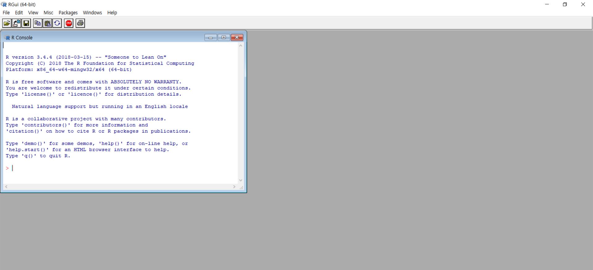
- R itself may look boring and tedious. However, we have a great helper called RStudio!
RStudio
- RStudio helps users to use and learn R easier.
- If you are using RStudio, this means you are using R.
- From now on, all tutorials will go with RStudio.
- Are you curious how it looks like on the screen? You’ll meet soon!
2. Time to become a friend: Installation
- To work with R, you need to download both R and RStudio.
- Please note that R should be downloaded first. Next, download RStudio.
R Installation
- Let’s go to this website.
- Go to a country close to you.
- Choose and click any one of the website links listed.
- Based on your operating system (Linux, Mac, Windows), click Download.
- If you use Linux, click Download R for Linux: Choose your Linux distribution (debian/, redhad/, suse/, ubuntu/) -> Open the terminal -> Run the installation command
- If you use Mac, click Download R for (Mac) OS X: Find the header ‘Latest release’ -> Click R-latest.version.pkg (or another version)
- If you use Windows, click Download R for Windows: Find ‘base’ under subdirectories -> Click ‘install R for the first time’ -> Click Download R latest.version (or another version) for Windows
RStudio installation
- This time, let’s go to this website.
- In this tutorial, we will download the most basic one. Thus, click DOWNLOAD under RStudio Desktop.
- If you use Linux: Find the header ‘All installers’ -> Under OS column, find your Linux distribution -> Look right: Click the corresponding download file
- If you encounter an error message during installation, try to install the public code-signing key before installation. To do that, under the ‘All Installers’ header, click ‘import RStudio’s public code-signing key’ -> Open the terminal -> Run the command under the headers ‘Obtaining the Public Key’ and ‘Validating Build Signature’
- If you use Mac: Find the header ‘All Installers’ -> Under OS column, find mac 10.13+ -> Look right: Click Rstudio-latest.version.dmg
- If you use Windows: Click DOWNLOAD RSTUDIO FOR WINDOWS
- If you use Linux: Find the header ‘All installers’ -> Under OS column, find your Linux distribution -> Look right: Click the corresponding download file
3. Eyes on the R: Screen structure
No ‘pane’, no gain!
- Note that the quote uses not ‘pain’ but ‘pane’. This implies that you will work with what is called ‘pane’ in RStudio without pain! When you finish the download and open the RStudio, the screen may look like this. What is your first impression of R?
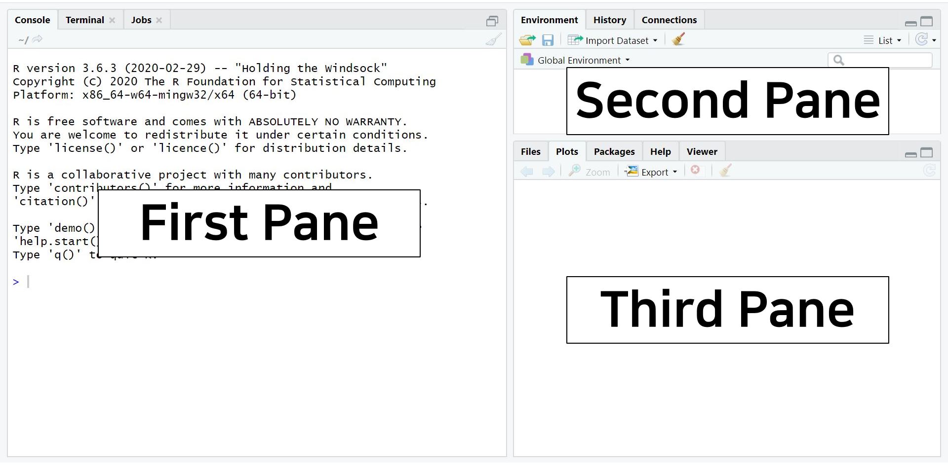
- There are three panes where each pane has a role. However, don’t be surprised because there is another pane that you will see if you open an R script. An R script is like a new document of Microsoft Word. When you open an R script, the hidden pane appears.
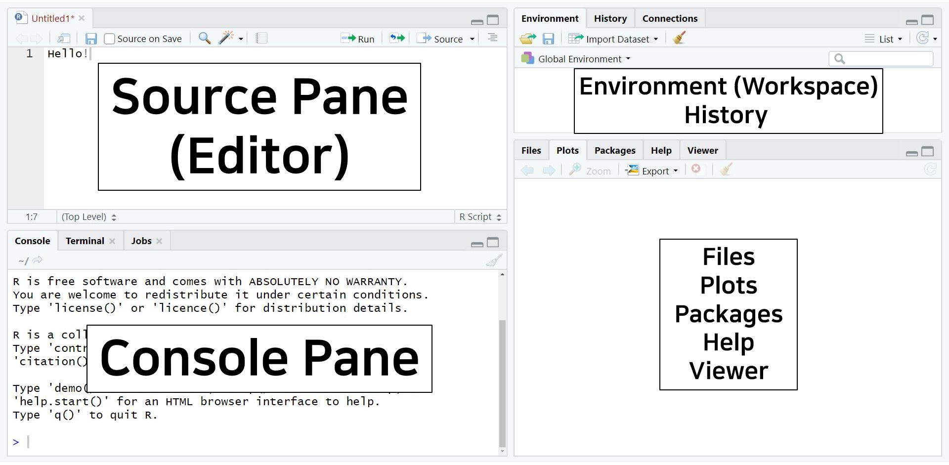
- Shall we open an R script? Click the icon with a plus sign on the paper. For you, I created a black square that indicates the icon: See the below!

- When you click the icon, the hidden pane appears.
- Can you see a new pane was added on the upper left side of the screen? It says hello to you!
- Are you scared of those four panes? No worries! This structure is beneficial. You can observe and perform all the processes simultaneously.
- Think about the situation in SPSS. You always have multiple pop-ups such as data editor, syntax editor, viewer, etc. Consequently, you have to switch one another to proceed with your analyses. In R, you can do everything all together on one screen. Thus, four panes make the work efficient (indeed, no ‘pain’)!
What do the four panes do?
- Out of four panes, the two on the left side are the panes you will use a lot.
- Source pane: located at the top left side of the screen. It is also called as an editor because we can command everything in this pane. Therefore, we will type code in the source pane.
- Console pane: located at the bottom left side of the screen. R will tell you what it is doing to us. In other words, we can communicate with R through the console pane. Besides, the output of statistical analyses is printed in the console pane.
- The panels on the right side of the screen contain various tabs. Among those tabs, it is worth looking at the Environment tab at the upper pane and the Plots tab at the lower pane.
- The Environment tab contains all the ‘materials’ we will use. You can always check your current materials under the environment tab. This environment tab is also called as a workspace.
- The Plots tab shows various graphs and figures we draw. If you click Zoom with the magnifying glass, you can see plots in a bigger size.
II. R you ready?
1. Take out your ‘main material’: Loading data
- Statistical analysis cannot happen without the data. In R, you can load the data in various ways. Let’s see the easiest way.
- If you did not download the dataset (
popular_regr_1) yet, click here.
Mouse clicks
- Click File -> Import Dataset -> Choose the type of dataset. In this tutorial, we will use the SPSS dataset. Thus, click ‘From SPSS’.
- Suddenly, you may encounter an Install Required Packages pop-up with a message that asks you whether you want to install the haven package now.
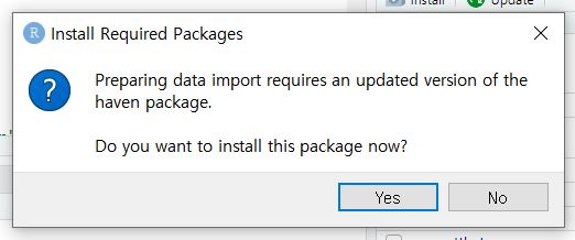
- Click ‘Yes’. Are you curious about what a package is? I recommend you to read ‘2. A gentle introduction to packages and functions’ in ‘V. Want moRe?’ later.
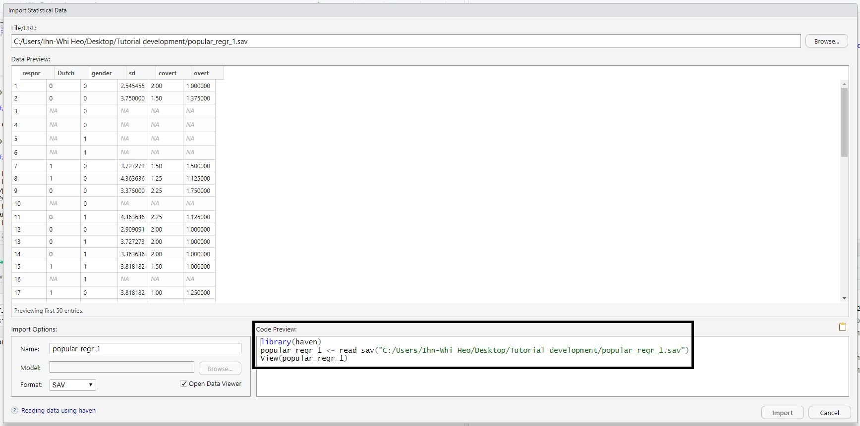
- Then, the Import Statistical Data pop-up appears -> See File/URL -> Click Browse at the right end -> Open your file
- You will see your data in the Data Preview.
- If you look at the Import Options, you can set the name of your data file and the format of it.
- All these ‘mouse-clicking’ procedures are being conducted in programming languages simultaneously. In the Code Preview, what we did in loading the data is expressed in terms of codes.
- Now, it’s time to load your data to R. How? Just click Import at the lower right side of the pop-up.
- In our example, the name of the dataset is
popular_regr_1.
“Can I try this again with R code by typing it in the source pane?”
- Good question. Of course! That is exactly what I am going to tell you.
2. This time as a programmer: Loading data with R code
- Let’s try to load the data with R code.
- Let’s start from opening the Import Statistical Data pop-up (Click File -> Import Dataset -> Choose the type of dataset -> From SPSS). Browse and open your data. At this moment, look at the Code Preview section. Can you see the R code? There are three lines of code where the first line is ‘library(haven)’.
- Drag all three lines and copy the code. Then, close the Import Statistical Data pop-up by clicking Cancel.
- Paste the codes you copied in the source pane. In the source pane, you contain the codes below.
- Please note that the code at the second line might look different depending on the location of the dataset in your computer. In general, the code should look like
popular_regr_1 <- read_sav("Location of the dataset in your computer/popular_regr_1.sav").
- Please note that the code at the second line might look different depending on the location of the dataset in your computer. In general, the code should look like
library(haven)
popular_regr_1 <- read_sav("C:/Users/Ihn-Whi Heo/Desktop/Tutorial development/popular_regr_1.sav")
View(popular_regr_1)- These are the codes you are going to use. At each line, press Ctrl and Enter together. Whenever you run those codes in each line, R is telling you that it is being conducted in the console pane. After all, this results in loading the same data you loaded via mouse clicks.
- As mentioned at the very first of this tutorial, R is open-source. Therefore, there are various ways to load the data. We will explain how to do in the other ways in ‘5. Packages and functions to load the data’ in ‘V. Want moRe?’.
III. ExploRe data
1. Looking into your data
- As you saw, you can type some R codes in the source pane and run the codes by pressing Ctrl and Enter together to make R work. If you look at the R codes we used in loading the data, there are such things as
read_sav()andView(). These are called functions. Functions in R enable us to perform many tasks efficiently. - When you use functions, you should type certain comments or inputs in the parentheses, which make the functions work. Those comments or inputs are called arguments. Let’s learn three new functions with their arguments. They are used in understanding the data.
head() function
- The dataset consists of rows and columns. If you would like to inspect the first several rows, the
head()function achieves your purpose. - For the
head()function, the number of arguments you will use is only one. What is it? It is ‘popular_regr_1’, which is the name of the dataset.
# Inspect the first several rows
head(popular_regr_1)
## # A tibble: 6 x 6
## respnr Dutch gender sd covert overt
## <dbl> <dbl> <dbl> <dbl> <dbl> <dbl>
## 1 1 0 0 2.55 2 1
## 2 2 0 0 3.75 1.5 1.38
## 3 3 NA 0 NA NA NA
## 4 4 NA 0 NA NA NA
## 5 5 NA 1 NA NA NA
## 6 6 NA 1 NA NA NA- “Wait, what is the number sign (#) in ‘# Inspect the first several rows?’” Don’t be surprised. We can use the number sign whenever we want to type text in the source pane. This is useful because we can identify what we are doing with the typed texts when there are many lines of code.
- Let’s run the code by pressing Ctrl and Enter together. R shows you the first six rows of the variables in the console pane.
- You may be curious about some NAs in the output. Those are the missing values. NA refers to ‘Not Available’.
str() function
- It is of interest to know what the types of variables are in the dataset. For example, if you want to run the analysis of variance (ANOVA), the independent variable should be categorical (i.e., factor), and we should check if it is the case.
- For this purpose, you need the
str()function where str refers to the structure. In running this function, you need one argument, which is the name of the dataset.
# Structure of the dataset
str(popular_regr_1)
## tibble [1,491 x 6] (S3: tbl_df/tbl/data.frame)
## $ respnr: num [1:1491] 1 2 3 4 5 6 7 8 9 10 ...
## ..- attr(*, "format.spss")= chr "F12.0"
## ..- attr(*, "display_width")= int 12
## $ Dutch : num [1:1491] 0 0 NA NA NA NA 1 1 0 NA ...
## ..- attr(*, "format.spss")= chr "F12.2"
## ..- attr(*, "display_width")= int 12
## $ gender: num [1:1491] 0 0 0 0 1 1 0 0 0 0 ...
## ..- attr(*, "format.spss")= chr "F12.0"
## ..- attr(*, "display_width")= int 12
## $ sd : num [1:1491] 2.55 3.75 NA NA NA ...
## ..- attr(*, "format.spss")= chr "F12.2"
## ..- attr(*, "display_width")= int 12
## $ covert: num [1:1491] 2 1.5 NA NA NA NA 1.5 1.25 2.25 NA ...
## ..- attr(*, "format.spss")= chr "F12.2"
## ..- attr(*, "display_width")= int 12
## $ overt : num [1:1491] 1 1.38 NA NA NA ...
## ..- attr(*, "format.spss")= chr "F12.2"
## ..- attr(*, "display_width")= int 12- According to the output in the console pane, the dataset consists of 1,491 rows and 6 columns. How do we know? Look at ‘tibble [1,491 x 6]’ where tibble simply refers to the data we are using. This implies that our dataset has 1,491 observations and 6 variables.
- It is written that respnr: num [1:1491] 1 2 3 4 5 6 7 8 9 10 … It means that the respnr variable is a number (abbreviated as num), and 1 is the value in the first row, 2 is the value in the second row, 3 is the value in the third row, and so on.
summary() function
- How can we know about the mean, median, minimum, and maximum of the variables of interest? You can get the descriptive statistics of the variables with
summary()function. Again, you only need one argument, which is the name of the dataset.
# Get descriptive statistics of the dataset
summary(popular_regr_1)
## respnr Dutch gender sd
## Min. : 1.0 Min. :0.0000 Min. : 0.0000 Min. :1.455
## 1st Qu.: 373.5 1st Qu.:0.0000 1st Qu.: 0.0000 1st Qu.:3.182
## Median :1203.0 Median :1.0000 Median : 0.0000 Median :3.636
## Mean :1045.1 Mean :0.5519 Mean : 0.9074 Mean :3.628
## 3rd Qu.:1652.5 3rd Qu.:1.0000 3rd Qu.: 1.0000 3rd Qu.:4.091
## Max. :2042.0 Max. :1.0000 Max. :99.0000 Max. :5.909
## NA's :257 NA's :145
## covert overt
## Min. :1.000 Min. :1.000
## 1st Qu.:1.500 1st Qu.:1.000
## Median :2.000 Median :1.250
## Mean :1.941 Mean :1.325
## 3rd Qu.:2.250 3rd Qu.:1.500
## Max. :3.750 Max. :3.125
## NA's :148 NA's :147- Let’s look at the output in the console pane. The descriptive statistics per variable is given. For example, for the adolescents’ socially desirable answering patterns (variable sd), the minimum value is 1.455, the median is 3.636, and the mean is 3.628.
2. How to visually inspect the data
- It is always a good idea to look into your data visually. For example, you would like to know the relationship between two specific variables in your data, the distribution of values, and more.
- For these purposes, three functions can visually help us understand the data. After you run these functions, the output appears in the Plots tab at the lower right pane.
hist() function
- Are you curious about how the values of one variable are distributed? Drawing a histogram is one way of examining the distribution. This is possible with the
hist()function with one argument that indicates the name of the variable in the dataset. - But wait, how can we specify a certain variable in our data? For example, if you want to draw the histogram of the variable sd, you can do this with the following code.
# Draw the histogram of the sd variable in the dataset
hist(popular_regr_1$sd)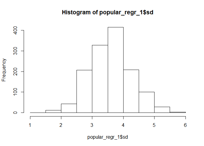
- There is a dollar ($) sign after the name of the data. In R, the dollar sign does not mean anything monetary. Rather, it can be interpreted as the specific element of the data. In this example, the popular_regr_1$sd refers to the variable, sd, of the data,
popular_regr_1. - An additional tip for you! You might be wondering how to change the plot title and the labels for the x-axis and the y-axis. With such arguments as ‘main =’, ‘xlab =’, and ‘ylab =’, we can simply make the plot more informative. The argument ‘main =’ is to edit the title, ‘xlab =’ is for the x-axis, and ‘ylab =’ is for the y-axis.
- Let’s change the title and the labels for two axes of the histogram above.
# Add title and labels for the histogram
hist(popular_regr_1$sd, main = "Histogram of sd", xlab = "sd", ylab = "Frequency")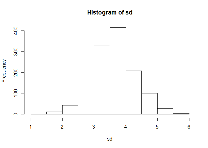
- Note that the quotation mark (“) is used to refer to the text we intend to change. Without the quotation mark, the change will not be applied.
boxplot() function
- This time, you may be interested in how the data are dispersed from the median and whether the outliers exist. You can solve your curiosity with the boxplot. In R, the
boxplot()function does this role. Let’s draw the boxplot of the variable, sd. Can you guess how to do this?
# Draw the boxplot of the sd variable in the dataset
boxplot(popular_regr_1$sd)
- This code means that you want to draw the boxplot of the variable, sd, in the dataset,
popular_regr_1. - In the boxplot, the dots above the upper whisker and below the lower whisker are outliers. Thus, we can say outliers exist in the variable, sd.
- Likewise, let’s add the title for the boxplot. You can do it with the ‘main =’ argument.
# Add title for the boxplot
boxplot(popular_regr_1$sd, main = "Boxplot of sd")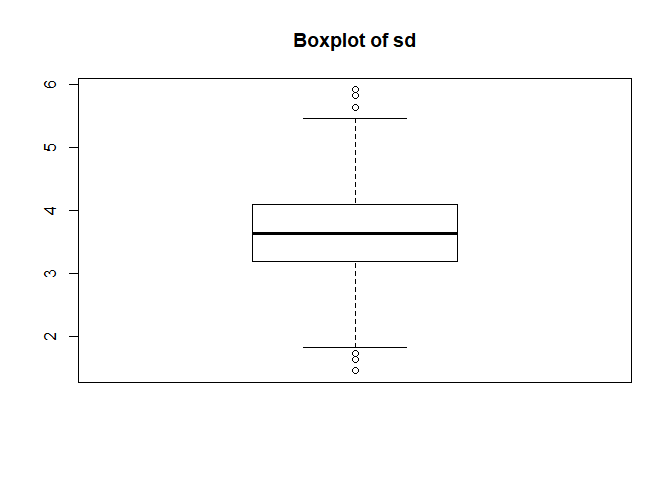
plot() function
- What if we are interested in visually investigating the relationship between two variables, sd and covert, in the data? The possible solution is to draw the scatterplot. Then, the
plot()function is what you need. This time, we need two arguments that indicate the names of the two variables in the dataset.- The first argument is ‘x =’. This indicates which variable will be located on the x-axis.
- The second argument is ‘y =’. This means which variable will be located on the y-axis.
# Draw the scatterplot between the sd variable (x-axis) and the covert variable (y-axis) in the dataset
plot(x = popular_regr_1$sd, y = popular_regr_1$covert)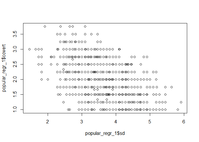
- This code gives you the scatterplot of the two variables, sd and covert. The variable, sd, is at the x-axis and the variable, covert, is at the y-axis.
- Depending on the arguments of the
plot()function, the function yields different kinds of plots. In this example, the plot function yielded a scatterplot. - Let’s imagine we want to give a title and change the axis labels for the plot. Can you guess what to do? Yes, use the arguments such as ‘main =’, ‘xlab =’, and ‘ylab =’!
# Add title and labels for the scatterplot
plot(popular_regr_1$sd, popular_regr_1$covert, main = "Scatterplot of sd and covert",
     xlab = "sd", ylab = "covert")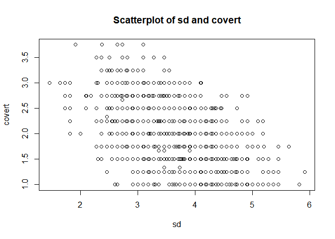
IV. Analyze and inteRpret data
- One of the strengths of R is its flexibility in running statistical analyses and producing graphical outputs. We will touch the four statistical analyses that are widely used: correlation analysis, multiple linear regression, t-test, and one-way analysis of variance.
- We assume that all the assumptions required for subsequent analyses are satisfied.
1. Correlation analysis
- If you want to test whether the correlation coefficient between the two variables is significant, you can use the
cor.test()function. - In our data, let’s examine whether the correlation coefficient between the covert and overt antisocial behavior (covert and overt) is significantly different from 0. We need two arguments that indicate the names of the two variables in the dataset.
# Test whether the correlation between covert and overt is significant
cor.test(popular_regr_1$covert, popular_regr_1$overt)
##
## Pearson's product-moment correlation
##
## data: popular_regr_1$covert and popular_regr_1$overt
## t = 15.318, df = 1341, p-value < 2.2e-16
## alternative hypothesis: true correlation is not equal to 0
## 95 percent confidence interval:
## 0.3394084 0.4304982
## sample estimates:
## cor
## 0.3858935- Your output appears in the console pane. The correlation coefficient is 0.39 (The actual output is 0.3858935, but we rounded to the second digit after the decimal point). Because the p-value is lower than .05 (2.2e-16 equals \(2.2 × 10^{-16}\), which is much lower than .05), we reject the null hypothesis that the correlation coefficient between covert and overt is 0.
- Here, the value of .05 refers to an alpha level. From now on, let’s use the alpha level of .05 since it is most commonly used!
2. Multiple linear regression
- When you are interested in predicting outcomes of a continuous variable with multiple continuous or categorical predictors, the multiple linear regression is the option you should choose.
- In R, we can use the
lm()function to regress a dependent variable on multiple independent variables. The lm refers to the linear model. - For illustrative purposes, let’s use adolescents’ socially desirable answering patterns (sd) as the dependent variable and overt and covert antisocial behavior (overt and covert) as independent variables.
- When you use the
lm()function for the multiple linear regression, you need to type the below code in the source pane.
# First, fit the linear model predicting sd with overt and covert with the lm() function
# Then, assign the fitted linear model to the ‘regression’
regression <- lm(sd ~ overt + covert, data = popular_regr_1)

# Result of the regression analysis
summary(regression)
##
## Call:
## lm(formula = sd ~ overt + covert, data = popular_regr_1)
##
## Residuals:
## Min 1Q Median 3Q Max
## -1.83617 -0.37325 -0.01874 0.36368 1.85524
##
## Coefficients:
## Estimate Std. Error t value Pr(>|t|)
## (Intercept) 4.99653 0.06618 75.497 < 2e-16 ***
## overt -0.29152 0.04573 -6.374 2.52e-10 ***
## covert -0.50711 0.02842 -17.846 < 2e-16 ***
## ---
## Signif. codes: 0 '***' 0.001 '**' 0.01 '*' 0.05 '.' 0.1 ' ' 1
##
## Residual standard error: 0.5742 on 1340 degrees of freedom
## (148 observations deleted due to missingness)
## Multiple R-squared: 0.2815, Adjusted R-squared: 0.2805
## F-statistic: 262.6 on 2 and 1340 DF, p-value: < 2.2e-16- You must be startled at complex signs and arguments. I feel you! Let’s learn step by step.
- First, you saw such new symbols as <- and ~. Second, the dollar sign ($) is disappeared in referring to the variables in the dataset.
- The left-headed arrow (<-) assigns functions or data to ‘something’. Technically, <- is called as an assignment operator. In our example, we assigned the
lm()function to ‘regression’. - The tilde (~) means ‘be regressed on’. Note that sd is the dependent variable, and overt and covert are the independent variables. This means that sd is predicted by overt and covert. We can equivalently express this as regressing sd on overt and covert. Thus, our example means that sd is regressed on overt and covert.
- The dollar sign ($) can be omitted with the usage of the ‘data =’ argument. The ‘data =’ argument automatically maps the variable names in the function to the corresponding variable names in the dataset. In our example, since we used the argument ‘data = popular_regr_1’, three variables (sd, overt, and covert) are automatically referred to as the variables in the
popular_regr_1dataset. How convenient and efficient!
- The left-headed arrow (<-) assigns functions or data to ‘something’. Technically, <- is called as an assignment operator. In our example, we assigned the
- Now, it’s time to run the code and see the results in the console pane.
- First, let’s focus on the values under the header ‘Coefficients’. These values are unstandardized regression coefficients (written under the Estimate column), standard errors (written under the Std. Error column), test-statistic (written under the t value column), and the p-value (written under the Pr(>|t|) column). What we have to look at is the Estimate column and Pr(>|t|) column.
- The unstandardized regression coefficient of overt is -0.29, and the p-value is lower than .05 (2.52e-10 equals \(2.52 × 10^{-10}\)). Again, we use the value of .05 as an alpha level. There are three asterisks at the right side of the p-value where the asterisk means the significance code. The three asterisks mean that the p-value is lower than 0.001. Therefore, the variable, overt, is a significant predictor with an alpha level of .05. If one unit of overt increases, the sd decreases 0.29 units.
- How about the unstandardized regression coefficient of covert? Look at the value under the Estimate column. The value is -0.51. This value is significant given the p-value lower than .05 (2e-16 means \(2 × 10^{-16}\)). The three asterisks show that the p-value is lower than 0.001. Thus, the variable, covert, is also a significant predictor, again with an alpha level of .05 (for your recap!). If one unit of covert increases, the sd decreases 0.51 unit.
- Second, let’s see the Multiple R-squared. The multiple R-squared is the proportion of variance of the outcome variable explained by the multiple predictors. Thus, the multiple R-squared value of 0.28 means that these two predictors explain 28% of the variance of sd.
- Finally, let’s look at the F-statistic. The F-statistic in the regression model tells you whether the model fits the data well. Can you find the p-value of the F-statistic at the right end? Because the p-value is lower than .05 (2.2e-16 means \(2.2 × 10^{-16}\)), this regression model fits significantly better than the model that does not have any independent variables.
3. t-test
- What if you want to examine whether the means of two certain groups are significantly different or not? For this purpose, we perform the t-test.
- Among variables in our data, let’s test whether the mean of the covert antisocial behavior (covert) and the mean of the overt antisocial behavior (overt) are significantly different. We can use the below code.
# Test whether the means of covert and overt are significantly different or not
t.test(popular_regr_1$covert, popular_regr_1$overt)
##
## Welch Two Sample t-test
##
## data: popular_regr_1$covert and popular_regr_1$overt
## t = 32.061, df = 2243.4, p-value < 2.2e-16
## alternative hypothesis: true difference in means is not equal to 0
## 95 percent confidence interval:
## 0.5781065 0.6534343
## sample estimates:
## mean of x mean of y
## 1.94068 1.32491- The p-value is lower than .05. Therefore, the two means of covert and overt are significantly different from each other.
4. One-way analysis of variance
- If researchers are interested in testing if the means are significantly different across different groups, they perform the analysis of variance. The
aov()function makes R perform ANOVA. - We will examine if the means of the covert antisocial behavior (covert) are different across respondents’ genders (gender). To do this, use the below code.
# Run the analysis of variance and assign the result to ‘anova’
anova <- aov(covert ~ factor(gender, exclude = c(99)), data = popular_regr_1)

# Result of the analysis of variance
summary(anova)
## Df Sum Sq Mean Sq F value Pr(>F)
## factor(gender, exclude = c(99)) 1 14.3 14.272 41.08 2.02e-10 ***
## Residuals 1335 463.8 0.347
## ---
## Signif. codes: 0 '***' 0.001 '**' 0.01 '*' 0.05 '.' 0.1 ' ' 1
## 154 observations deleted due to missingness- Did you find that we assigned the result of
aov()function to ‘anova’? Did you also catch that we omitted the dollar ($) sign when referring to the variable names thanks to the ‘data =’ argument? - It is likely that you should be surprised at the usage of ‘factor(gender, exclude = c(99))’. Let’s see what it is!
- Do you remember that the independent variable in the ANOVA should be a factor, which is a categorical variable? Using ‘factor’ is to treat gender variable as a categorical variable.
- What is ‘exclude = c(99)’? This is to filter the ‘99’ category out from the analysis. Otherwise, R will treat 99 as an independent category, which is not the case.
- The p-value of gender is 2.02e-10 (2.02e-10 means \(2.02 × 10^{-10}\)), which is lower than .05. Therefore, we reject the null hypothesis of no group mean difference. In other words, we find a statistically significant difference in means across the two genders.
Congratulations!
- Are you enjoying the tutorial? Hope so! If you’ve successfully finished everything mentioned until now, you are standing at a very good starting point for further advanced analyses.
- From now on, let us tell you some helpful additional tips.
V. Want moRe?
1. Not r but R: R is case sensitive!
- R distinguishes upper and lower letters. Therefore, you should be careful in typing any code in the source pane. As we will see soon, examscore and EXAMSCORE are different.
- This case sensitivity also affects function. If you use
MEAN()to get the mean of the variable, the function does not work, and the console pane gives you an error message. Thus, you should use themean()function to calculate the mean. - Let’s see the example below.
# Assign a set of numbers (80, 90, 100, 75, 60, 85, 95) to ‘examscore’
# c() is the function to combine the arguments in the parenthesis where c stands for concatenate
examscore <- c(80, 90, 100, 75, 60, 85, 95)

# Print the values of examscore
print(examscore)
## [1] 80 90 100 75 60 85 95# Print the values of EXAMSCORE
print(EXAMSCORE)## Error in print(EXAMSCORE): object 'EXAMSCORE' not found- If you print the examsocre, R gives you 7 values that we assigned to examscore. However, if you try to print the EXAMSCORE, R says ‘Error in print(EXAMSCORE) : object ‘EXAMSCORE’ not found’ in the console pane.
- You may have a question about what the object is. Simply put, an object in R is every entity that is created, manipulated, or used. Objects can be variables, an array of numbers, datasets, functions, and other structures. Can you remember that the Environment tab contains all the ‘materials’ we use? These materials are objects! In other words, those exist in the Environment tab are all objects you are using.
# Compute the mean of examscore
mean(examscore)
## [1] 83.57143# MEAN() function to calculate the mean of examscore does not work
MEAN(examscore)## Error in MEAN(examscore): could not find function "MEAN"# Compute the median of examscore
median(examscore)## [1] 85- The
mean()function calculates and gives the mean of examscore, which is 83.57. On the other hand, theMEAN()function cannot calculate the mean of examscore, and the R says ‘Error in MEAN(examscore) : could not find function “MEAN”’.
2. A gentle introduction to packages and functions
- There are 15,551 packages and the enormous number of functions in R as of April 1, 2020 (I’m not fooling you!). Some packages and functions are in-built when you first download R. Others are ones made by other people.
- The
read_sav()function we used in loading the data is part of thehavenpackage. The package is a collection of functions and datasets. If you want to download thehavenpackage and load thehavenpackage to use, you have to useinstall.packages()function andlibrary()function. - Before I show you the code, I want to tell you that you already installed the
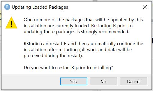
havenpackage by mouse clicking! Can you recall that you encountered an Install Required Package pop-up that asked you whether you were going to install thehavenpackage? Because you said Yes, the package has been already installed. - Accordingly, you will see an Updating Loaded Packages pop-up like the below picture if you run the upcoming code for downloading and loading the
havenpackage. If you do not want to update thehavenpackage, simply click Cancel. Otherwise, click Yes if you want to restart R before installation or No if you do not want to restart R before installation.
# Download the haven package
install.packages("haven")

# Load the downloaded haven package
library(haven)- Note that we have to specify the name of the package we want to download in quotation mark (“).
- For now, we will try to download other packages and functions to load the data rather than
read_sav()function in thehavenpackage. Before that, there is an important stage you have to conduct: setting the working directory.
3. Bring your bag: Working directory
- Before you go to class, you prepare for your books, pens, and laptop (in my case, snack as well!) in your bag. After you arrive in the classroom, you pull out those things from the bag. This is the same in R! When you want to analyze data, you have to prepare for your data in a special bag for R. This bag is called a working directory.
- “But wait, how can I bring my bag?” It’s easy. You do not need to go home. You only use your mouse.
Mouse clicks
- Go to the bottom right pane -> Choose the Files tab -> Click ‘…’ at the right end -> Click the folder that contains your data -> Click Open -> Click More with the toothed wheel -> Click ‘Set as Working Directory’
Check your current working directory!
- Please look at the console pane. Right after you’ve set the working directory, R tells you where it set the working directory!
4. All about working directory with R code
- Previously, we set the working directory with some mouse clicks. Not surprisingly, it is also possible to set the working directory with R codes. In this situation, we use the
setwd()function where wd refers to the working directory. On the other hand, we can check the current working directory with thegetwd()function. - Before running the
setwd()function, we need to know where the data file is because you have to set your working directory to the place that contains your data! You can know the ‘address’ of the data file by right-clicking the data file you will use and asking for Properties. Then, just copy the location of the file within the parenthesis of thesetwd(). - However, there are two things to consider. First, the address you copied should be within the quotation mark (“). Second, you have to change from the backslash (\) into the slash (/).
- The codes below show the whole process you have to do to set the working directory and get the working directory you set.
# Set the working directory
setwd("C:/Users/UserName/Desktop/Your Folder")

# Check the working directory
getwd()
5. Packages and functions to load the data
- The reason why I explained to you how to set and get the working directory before providing other packages and functions in loading the data is that the following functions will not work unless you set the working directory correctly.
- However, we now know how to prepare our special bag, called the working directory, that contains our data. It’s time to proceed to the examples of loading data using other packages and functions.
Some in-built functions
- If your data are stored as .csv, .txt, or .dat files, there are two in-built functions to load the data. If the data are separated with commas, the file is in .csv. On the other hand, the data in .txt or .dat files are separated with tabs. In the former case, you can use
read.csv()function. In the latter case,read.delim()is the option.
# Read the data in .csv file
data <- read.csv(file = "FileName.Extension", header = TRUE)

# Read the data in .dat file
data <- read.delim(file = "FileName.Extension", header = TRUE)- The FileName in the quotation mark (“) should equal to the actual file name with extension. In the preceding examples for exploring, analyzing, and interpreting data, the name of our dataset was
popular_regr_1, which was stored as an SPSS file. Consequently, we should type popular_regr_1.sav in the quotation mark. That is, the ‘file =’ argument should look like ‘file = “popular_regr_1.sav”’. - There is a new argument: header = TRUE. That argument means that we will use the first row of the dataset as the column names. If you do not want to do that, use ‘header = FALSE’.
- If the file name is too long or difficult to type, there is a useful function that gives you the ‘Select file’ pop-up. Then, you can simply choose the file you want to open in R with the mouse clicks. This is possible with the
file.choose()function.
# Choose the .csv file with the ‘Select file’ pop-up
data <- read.csv(file = file.choose(), header = TRUE)
foreign package
- Many researchers work with SPSS data, which is stored as a .sav file. For this purpose, there is a special function called
read.spss()in the foreign package. Theread.spss()function enables you to load the .sav file directly.
# Install and load the foreign package
install.packages("foreign")
library(foreign)

# Load the .sav file
data <- read.spss(file = "FileName.Extension", to.data.frame = TRUE)
data <- read.spss(file = file.choose(), to.data.frame = TRUE)- There is another new argument: to.data.frame = TRUE. This argument means that you will load the dataset as a data frame. A data frame consists of rows and columns. When you set the argument as ‘to.data.frame = FALSE’, R reads the data as a list of variable names in the dataset.
- In either way, you can perform statistical analyses such as getting the descriptive statistics. However, to manage the structure of the dataset by transforming the rows or columns, it is convenient to treat the data as a data frame. Therefore, I recommend you to use ‘to.data.frame = TRUE’ argument.
6. Save the best for last: Advisors inside and outside of R
- Congratulations! We are at the very last part of this tutorial. Now, you earned quite a lot of knowledge about R.
- However, are you unclear about which arguments are necessary to run the function? Are you nervous because you do not know which packages or functions to use in some situations? Are you worried about any potential problem you will face while doing R? No worries! Advisors are everywhere. This last part of the tutorial is reserved for teaching you how to search for everything for yourself. We promise this is very valuable for beginners in R.
Advisors inside of R: Use ?, ??, and the Help tab
- The ? and ?? above are not errors! They are useful tools that can help you.
- If you hope to know which arguments are necessary to run specific functions and want to see examples, you can type ? (question mark) in front of the function name without any space between ? and the name of a function.
- For instance, if you are interested in knowing the arguments of the
read_sav()function, you can type like below.
# Search for information about read_sav() function
?read_sav

# Usage of the help() function gives you the same information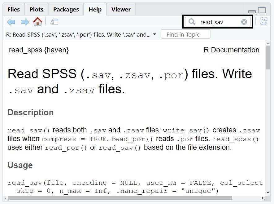
help(read_sav)- Then, the lower right pane shows you the information about the function in the Help tab.
- Searching for information about the function can also be done directly at the Help tab. Simply type read_csv in the right blank after the magnifying glass and start searching like the below picture!
- When you type the question mark twice (??) in front of the function without any space, the R searches your function in the Comprehensive R Archive Network (CRAN). CRAN is the main repository for R packages and functions.
# Search the function in the Comprehensive R Archive Network (CRAN)
??read_sav- The search result tells you the name of the package that contains the function you searched with ??.
Advisors outside of R: Stack Exchange, Stack Overflow, and Googling tips
- Advisors exist even outside of R! The three main sources are such websites as Stack Exchange, Stack Overflow, and Google.
- Stack Exchange is a collection or a network of websites for questions and answers for diverse topics. The topics include not only something statistical such as programming and mathematics but also contain others like software engineering, Linux, computer science, and more.
- Stack Overflow is one of the websites that exist in Stack Exchange. Stack Overflow is geared for programming, coding, packages, and functions. In other words, you can find and ask for anything relevant to your statistics within R.
- For example, if you want to know how to read the SPSS file into R, just type ‘Reading .sav file into R’ to search for any relevant information like the below picture.

- Googling on Google always gives you helpful websites, blogs, posts, or whatever that can be useful for your situation. I strongly recommend these two suggestions to find the solution to your problems: use prefix ‘r’ or suffix ‘in r’ when googling. The prefix ‘r’ and the suffix ‘in r’ are so magical that they will give you suitable information.
- Again, let’s imagine we want to find solutions concerning how to read the spss file in r. For this purpose, you can google either ‘r spss import’ with the prefix ‘r’ or ‘read spss file in r’ with the suffix ‘in r’
- As another instance, are you curious about how to calculate the variance in R? You may google either ‘r variance calculation’ or ‘how to compute variance in r’.
- As the final example, imagine you want to search for some functions that can calculate the power. You can google either ‘r power calculation function’ or ‘power calculation function in r’.
- In the end, learning how to search by oneself is the most productive and active way to solve problems for R programming. Thus, please enjoy googling that will solve your problems shortly.
- Last but not least, I wish you can answer to the questions from the R newbies in the near future!
References
R Core Team. (2020). R: A Language and Environment for Statistical Computing, Vienna, Austria. https://www.R-project.org/
Van de Schoot, R. (2020). Popularity Dataset for Online Stats Training [Data set]. Zenodo. https://doi.org/10.5281/zenodo.3962123
Van de Schoot, R., Van der Velden, F., Boom, J., & Brugman, D. (2010). Can at-risk young adolescents be popular and anti-social? Sociometric status groups, anti-social behaviour, gender and ethnic background. Journal of adolescence, 33(5), 583-592. https://doi.org/10.1016/j.adolescence.2009.12.004
Venables, W. N., Smith, D. M., & R Core Team. (2020). An introduction to R. https://cran.r-project.org/doc/manuals/r-release/R-intro.pdf