Advanced Bayesian regression in jamovi
Ihnwhi Heo and Rens van de Schoot
Department of Methodology and Statistics, Utrecht University
Last modified: 02 December 2020
This tutorial explains how to interpret the more advanced output and to set different prior specifications in conducting Bayesian regression analyses in jamovi (The jamovi project, 2020). We guide you to various options in the options panel and introduce concepts including Bayesian model averaging, prior model probability, posterior model probability, inclusion Bayes factor, and posterior exclusion probability. After the tutorial, we expect readers can deeply understand the Bayesian regression and perform it to answer substantive research questions.
For readers who need the basics of jamovi, we suggest following jamovi for beginners. For readers who want to learn the nuts and bolts of Bayesian analyses in jamovi, we recommend reading jamovi for Bayesian analyses with default priors. The current tutorial assumes that readers are prepared for backgrounds to dive into advanced Bayesian regression analysis.
Since we continuously improve the tutorials, let us know if you discover mistakes, or if you have additional resources we can refer to. If you want to be the first to be informed about updates, follow Rens on Twitter.
How to cite this tutorial in APA style
Heo, I., & Van de Schoot, R. (2020, December). Tutorial: Advanced Bayesian regression in jamovi. Zenodo. https://doi.org/10.5281/zenodo.4117884
PhD-Delays Dataset
We will use a phd-delay dataset (Van de Schoot, 2020) from Van de Schoot, Yerkes, Mouw, and Sonneveld (2013). To download the dataset, click here.
The dataset is based on a study that asks Ph.D. recipients how long it took them to complete their Ph.D. projects (n = 333). It turned out that the Ph.D. recipients took an average of 59.8 months to finish their Ph.D. trajectory.
For more information on the sample, instruments, methodology, and research context, we refer interested readers to the paper (see references). A brief description of the variables in the dataset follows. The variable names in the table below will be used in the tutorial, henceforth.
| Variable name | Description |
|---|---|
| B3_difference_extra | The difference between planned and actual project time in months |
| E4_having_child | Whether there are any children under the age of 18 living in the household (0 = no, 1 = yes) |
| E21_sex | Respondents’ gender (0 = female, 1 = male) |
| E22_Age | Respondents’ age |
| E22_Age_Squared | Respondents’ age-squared |
How to cite the dataset in APA style
Van de Schoot, R. (2020). PhD-delay Dataset for Online Stats Training [Data set]. Zenodo. https://doi.org/10.5281/zenodo.3999424
I. Setting a goal: A research question
- Earning a Ph.D. degree is a long and enduring process. Many factors are involved in timely completion, abrupt termination, or some delay of the Ph.D. life. For the current tutorial, we investigate how age is related to the Ph.D. delay.
- Let’s think about the relationship between age and Ph.D. delay. Do you think they are linearly related? Are there any different ideas such that the age is non-linearly associated with the delay? We expect the relationship between the completion time and age are non-linear. This might be because, at a certain point in your life (say mid-thirties), family life takes up more of your time compared to when you are in the twenties.
- To that end, we investigate whether the age of the Ph.D. recipients predicts a delay in their Ph.D. projects. The regression model is consequently the one we should adopt to answer the research question. We use the difference variable (B3_difference_extra) as the dependent variable and the age (E22_Age) and the age-squared (E22_Age_Squared) as the independent variables for the regression model.
II. Dataset, from A to Z
1. Loading data
- The statistical analysis goes together with the data. Click here to download the dataset necessary for our tutorial.
- There are two ways to load data in jamovi: one is from your personal computer and the other is from the in-built data library.
- If you are not familiar with loading the data, please go to jamovi for beginners and see how to load data.
- When you successfully load the dataset, the column names should be identical to the variable names in the dataset.

2. Exploring and checking out data
- It is always a good habit to explore your data once loaded. We can check out via either descriptive statistics or data visualization.
- If you are not familiar with exploring data, please go to jamovi for beginners and see how to inspect data.
Descriptive statistics
- Let’s take a look at the descriptive statistics of the variables to see if all the data points make substantive sense.
- Go to the Analyses ribbon -> Click Exploration -> Descriptives -> Move all variables to the Variables section on the right -> Check Frequency tables -> Click Statistics bar -> For a better inspection, check additional descriptive statistics (Std. deviation and S. E. Mean under Dispersion; Skewness and Kurtosis under Distribution)

- For all the variables, the sample size is 333 without any missing values.
- For the difference variable (B3_difference_extra), the mean and the standard error of the mean (S. E. Mean) are 9.97 and 0.791.
- For the age variable (E22_Age), the mean and the standard error of the mean are 31.7 and 0.376.
- For the age-squared variable (E22_Age_Squared), the mean and the standard error of the mean are 1050 and 36.0.
- For the dichotomous variables (E4_having_child and E21_sex), frequency tables are presented.
- Given the descriptive statistics, all the data points make sense substantively.
Data visualization
- Let’s draw a scatter plot to visually understand the relationship between age and the delay. To do that, the scatr module should be installed from the jamovi library (Do you remember that you can do that with the plus button?). We assume that the readers know how to install the module and are prepared for the scatr module.
- If you are not familiar with installing modules, please go to jamovi for beginners and see the steps to install modules.
- Go to the analyses ribbon -> Click Exploration -> Scatterplot under the scatr header
- Move E22_Age to the X-Axis section and B3_difference_extra to the Y-Axis section. The reason for locating the age variable and the difference variable to the x-axis and y-axis, respectively, is because we regress the difference variable on the age variable to answer our research question.
- To first examine a non-linear relationship between the difference variable and the age variable, check Smooth under Regression Line in the options panel.
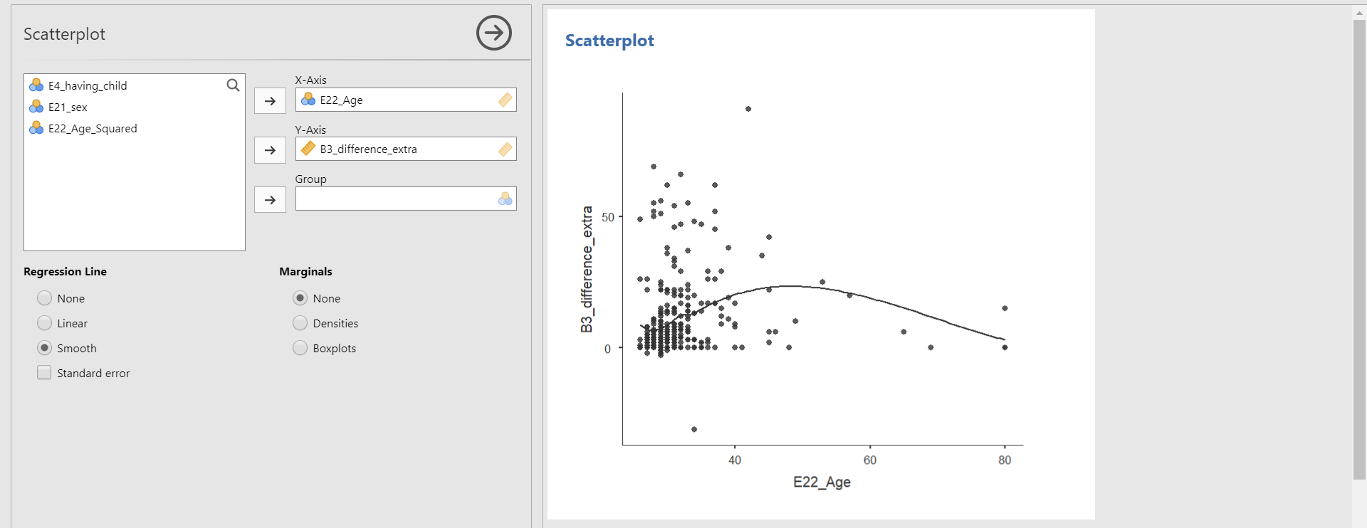
- From the scatter plot with a non-linear line, we can detect the non-linear relationship between the two variables.
- This time, let’s take a look at the linear relationship by drawing the linear regression line. Uncheck Smooth and check Linear under the Regression Line. Do you see the linear line?

III. Intermezzo: Parameter estimation and hypothesis testing from a Bayesian viewpoint
1. Bayesian parameter estimation
- A noticeable characteristic of Bayesian statistics is that the prior distributions of parameters are combined with the likelihood of data to update the prior distributions to the posterior distributions (see Van de Schoot et al., 2014 for introduction and application of Bayesian analysis). The updated posterior distributions are materials for Bayesian statistical inference. This logic implies the crucial role of prior distributions in doing Bayesian statistics!
- In our regression model, parameters are the intercept, two regression coefficients, and residual variance. Therefore, we should respectively specify the prior distributions for the intercept, two regression coefficients, and residual variance.
- Please note that we leave the discussion about priors for the intercept and the residual variance untouched in this exercise. We thus consider the prior distributions for the regression coefficients only.
- Let’s think about the model under consideration to see what the regression coefficients are. The regression formula for the current example can be written as: \(Difference = b_{0} + b_{Age} * X_{Age} + b_{Age-squared} * X_{Age-squared}\)
- You an see that the regression coefficients are \(b_{Age}\) and \(b_{Age-squared}\) whereas \(b_{0}\) is the intercept.
- The regression coefficients you will see later in the results panel are summaries of the posterior distributions of these two regression coefficients.
2. Bayesian hypothesis testing.
- Bayesian hypothesis testing focuses on which hypothesis receives relatively more support from the observed data. This is quantified by the Bayes factor (Kass & Rafter, 1995).
- Say we are considering two hypotheses: the null hypothesis (\(H_{0}\)) and the alternative hypothesis (\(H_{1}\)). If the Bayes factor in favor of the alternative hypothesis (i.e., \(BF_{10}\)) is 15, this means that the support in the observed data is about fifteen times larger for the alternative hypothesis than for the null hypothesis. In this way, how likely the data are to be observed among competing hypotheses is expressed in terms of the Bayes factor.
- Please note that we do not use words such as significant and p-value in Bayesian statistics. They are the terms used under the frequentist framework.
3. Obtaining reproducible results with a seed value
- Bayesian inference is based on the posterior distribution of parameters after taking into account the likelihood of data and the prior distribution. The likelihood and the prior are in the form of mathematical functions.
- The potential problem that could arise is that, usually, the posterior distribution is hard to get by analytical calculations (see Chapter 5 and Chapter 6 in Kruschke, 2014 for information about conjugate and non-conjugate prior). To solve this issue, Bayesian statistics uses the random number generator to approximate the posterior distribution. Due to generating random numbers, results from Bayesian analyses are slightly different each time we run Bayesian analyses.
- Surprisingly, this is not completely random such that each software has its hidden rule that the sequence of random numbers is generated! We can thus say the software is based on a pseudorandom number generator. The idea is that, whenever a certain number is fed as an input to the generator, the software produces the same sequence of pseudorandom numbers. Therefore, researchers and statisticians feed a specific number to the statistical software to make it reproduce the same outputs. For more information about setting seed values for Bayesian statistics, see Chapter 7 in Kruschke (2014).
- This tutorial is based on the jsq module version 1.0.1 where setting a seed value is not supported at the moment. Therefore, we kindly advise readers to be aware of this concern and not to be surprised if the Bayesian analyses with jamovi do not produce the same results each time.
IV. Bayesian regression analyses with default priors
- Please note that the jsq module should be installed on jamovi to perform Bayesian analyses. We assume that readers are prepared for the jsq module and are familiar with performing Bayesian statistical analyses.
- If you are not familiar with installing modules, please go to jamovi for beginners and check procedures to download modules.
- If you are not familiar with performing Bayesian analyses with default priors, please go to jamovi for Bayesian analyses with default priors and follow the steps to analyze the data.
- For subsequent analyses, let’s assume all the necessary assumptions are satisfied.
1. In-depth interpretations of the Bayesian regression output
A review for interpreting the posterior summary for default priors settings
- Move B3_difference_extra to the Dependent Variable section and E22_Age and E22_Age_Squared to the Covariates section. In the options panel, check Posterior summary under Output. Next, choose Model from Best model to Model averaged.
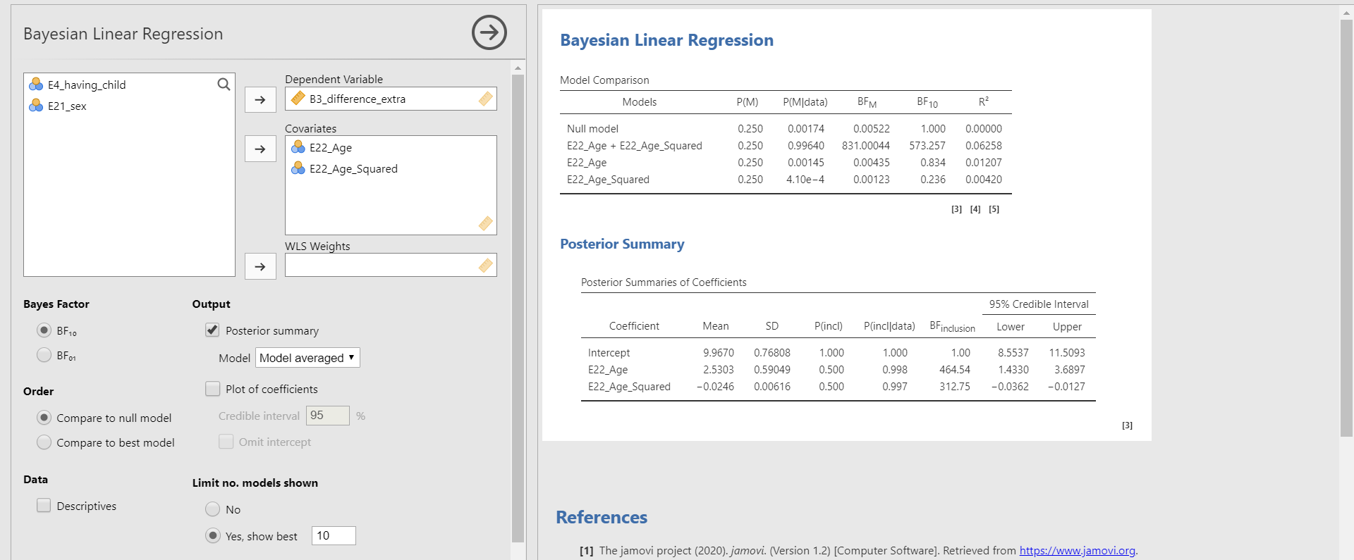
- What we need to look at to interpret the results is the Posterior Summaries of Coefficients table in the results panel. The table presents the summary of regression coefficients after taking into account the default priors for age and age-squared variable and the likelihood of data.
- The posterior mean of the regression coefficient of age is about 2.530. This can be interpreted that a one-year increase in age adds about 2.530 delays in Ph.D. projects, on average. The 95% credible interval of [1.4330, 3.6897] indicates that we are 95% sure that the regression coefficient of age lies within the corresponding interval in the population. Also, 0 is not included in the interval. Thus, it is fairly sure that there is an effect of the age variable in predicting the delay.
- The posterior mean of the regression coefficient of age-squared is about -0.025. We can interpret this value such that a one-unit increase of the age-squared variable leads to a decrease of 0.025 units in the Ph.D. delay, on average. The 95% credible interval of age-squared is [-0.0362, -0.0127], which means that there is a 95% probability that the regression coefficient of age-squared lies in the population with the corresponding credible interval. Do you notice that the 95% credible interval does not include 0? This shows the evidence of the effect of age in predicting the Ph.D. delay.
Bayesian model-averaged parameter estimates
- One important fact that we skipped in interpreting the parameter estimates above is that they are model-averaged results of parameter estimation as we selected Model averaged under Output in the options panel. Do you see the word Model averaged?
- To understand what the idea of the model-averaging is, recall the regression model we constructed for the current example: \(Difference = b_{0} + b_{Age} * X_{Age} + b_{Age-squared} * X_{Age-squared}\)
- We based our statistical inference on this single regression model that includes the two predictors, namely age and age-squared. This kind of inference with the single model, however, has inherent risk in the uncertainties of model selection.
- What if the model that does not contain the age variable also provides a good fit to the data and gives substantively different estimates? What if the model that does not contain the age-squared variable is more feasible than the model that contains both predictors after observing the data?
- Consequently, the parameter estimation based on the single model might give misleading results (Hoeting, Madigan, Raftery, & Volinsky, 1999; Hinne, Gronau, Van de Bergh, & Wagenmakers, 2020; Van de Bergh et al., 2020). Bayesian model averaging can solve this issue such that one can get parameter estimates after considering all the candidate models (i.e., the number of models that one can construct given the predictors).
- Okay, this sounds like a great idea. However, how do we average estimates across the candidate models? The solution is to average estimates based on the posterior model probabilities. In Bayesian statistics, the probability of the model given the observed data is called the posterior model probability. Posterior model probability is interpreted as the relative probability in favor of the model under consideration after observing the data.
- Then, how do we know how probable each candidate model is before seeing the data? The answer is to assign the prior model probabilities to each candidate model. Prior model probability is the relative plausibility of the models under consideration before observing data. That is, prior model probability tells us how probable the model is before we see data.
- In jamovi, we can set the prior model probability in the options panel. If you click the Advanced Options bar, there is Model prior. By default, the uniform distribution is chosen. This means that, under the uniform model prior, we assume all models are equally likely a priori. Hoeting, Madigan, Raftery, and Volinsky (1999) illustrated this choice as neutral.
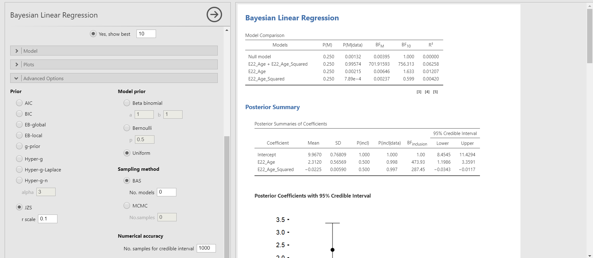
- In our example where there are two predictors, there exist four candidate models: the model that does not contain any predictors (also called the null model), the model that only contains the age variable, the model that only contains the age-squared variable, and the model that contains both predictors. In the results panel, jamovi provides these candidate models. Where? Look at the table under Model Comparison! Thus, the Posterior Summaries of Coefficients table provides parameter estimates after taking into account all the candidate models in the Model Comparison table.
Inclusion Bayes factor
- At this moment, we would like to introduce the concept of the inclusion Bayes factor (\(BF_{inclusion}\)), one of the columns in the Posterior Summaries of Coefficients table.
- The inclusion Bayes factor quantifies how much the observed data are more probable under models that include a particular predictor relative to the models that do not contain that particular predictor.
- For the age variable, the inclusion Bayes factor is 464.54. This implies that the model that contains the age variable is, on average, about 465 times more likely than the model without the age variable when we consider all the candidate models.
- For the age-squared variable, the inclusion Bayes factor is 312.75. We can interpret this value that, across all the candidate models, the model with the age-squared variable is, on average, about 313 times more likely than the model without the age-squared variable.
Parameter estimates for the best model
- You might want to examine the parameter estimates under the best single model that is the most probable given the observed data. We only need to change the ‘Model averaged’ option into the ‘Best model’ option.
- The interpretation of the Posterior Summaries of Coefficients table is the same as above except for the fact that now the estimates are not averaged but from the best model.

- “What is the best model, in this case?” This is a very nice question! The best model is the most probable or feasible model after observing the data. To choose that model, the probability of the model given the observed data (i.e., the posterior model probability) should be the highest.
- In the Model Comparison table, the column of P(M|data) indicates the posterior model probability. In our example, the model that contains both predictors has the highest posterior model probability, which is about 0.996 (almost 1). Then, what is P(M)? It denotes the prior model probability that we have explained before.
- According to the Model Comparison table, for the regression model that contains both predictors (i.e., E22_Age + E22_Age_Squared), the probability of the model has increased from 25% to 99.6%, after observing the data.
- The \(R^{2}\) we see in the last column of the Model Comparison table is the proportion of variance explained by the predictors in the model. The model that contains both predictors has the highest \(R^{2}\) of about 0.063 among all the candidate models. The \(R^{2}\) of 0.063 means that the age and the age-squared variable explains 6.3% of the variance in the Ph.D. delay.
- In the upcoming sections, we keep using the model-averaged estimates.
2. A graphical investigation for posterior summaries
- For the Posterior Summary in the results panel, we can take a look at the same information in a visual way. This way enables us to understand the results with more intuition.
Plot of coefficients
- The Posterior Summaries of Coefficients table provides many numbers, but we are mainly interested in the posterior mean and the 95% credible interval of parameters. The plot of coefficients helps us to figure out that information.
- Click Plots of coefficients under Output in the options panel -> Check Omit intercept
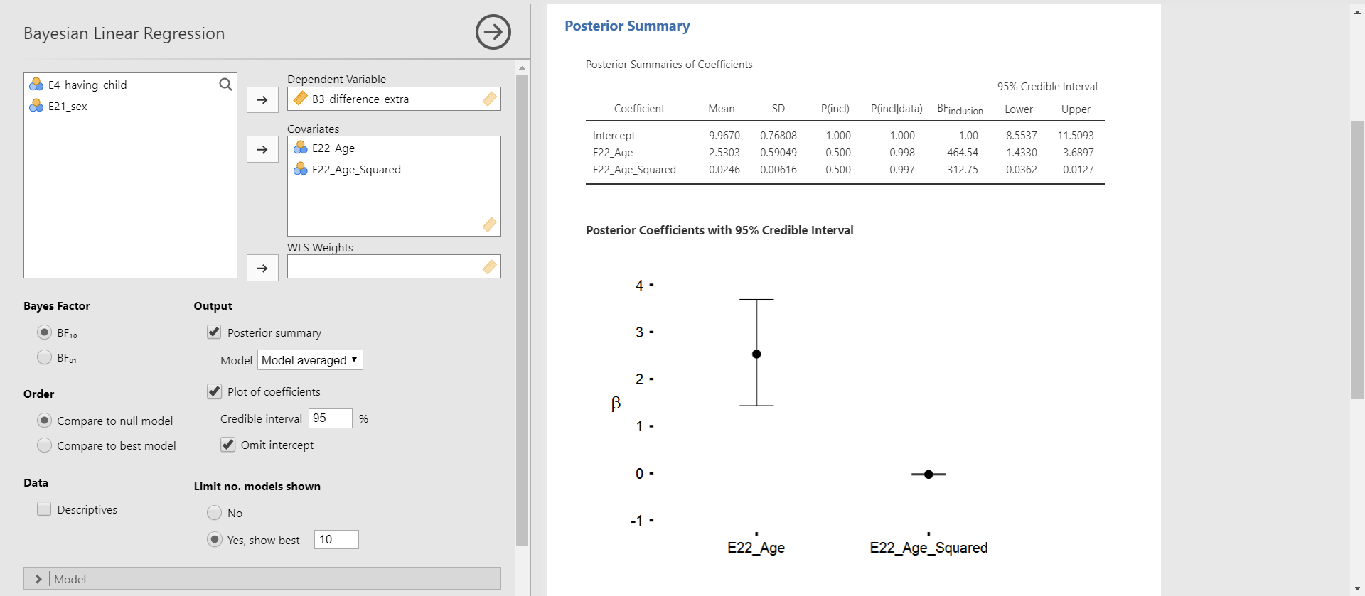
- You can see the Posterior Coefficients with 95% Credible Interval in the results panel. This plot shows the posterior distributions of both regression coefficients in the current model.
- The black round dot corresponds to the posterior mean of each regression coefficient. The upper and lower whisker surrounds the 95% credible interval. For the age variable, the 95% credible interval does not include 0. For the age-squared variable, it is difficult to clearly identify whether 0 is included in the 95% credible interval because the interval is very narrow and close to 0. In this case, we should refer to the numbers in the Posterior Summaries of Coefficients table.
- “Why did we decide to omit the intercept in the plot?” This is a great question! In our regression example, the intercept means the average of the Ph.D. delay when the values of age and age-squared are 0. We previously saw from the descriptive statistics that the mean and the standard error of the mean for the age variable are 31.7 and 0.376. Thus, interpreting the meaning of the intercept in this context is meaningless. Rather, plotting the posterior distributions for the regression coefficients of age and age-squared is more informative.
Marginal posterior distribution
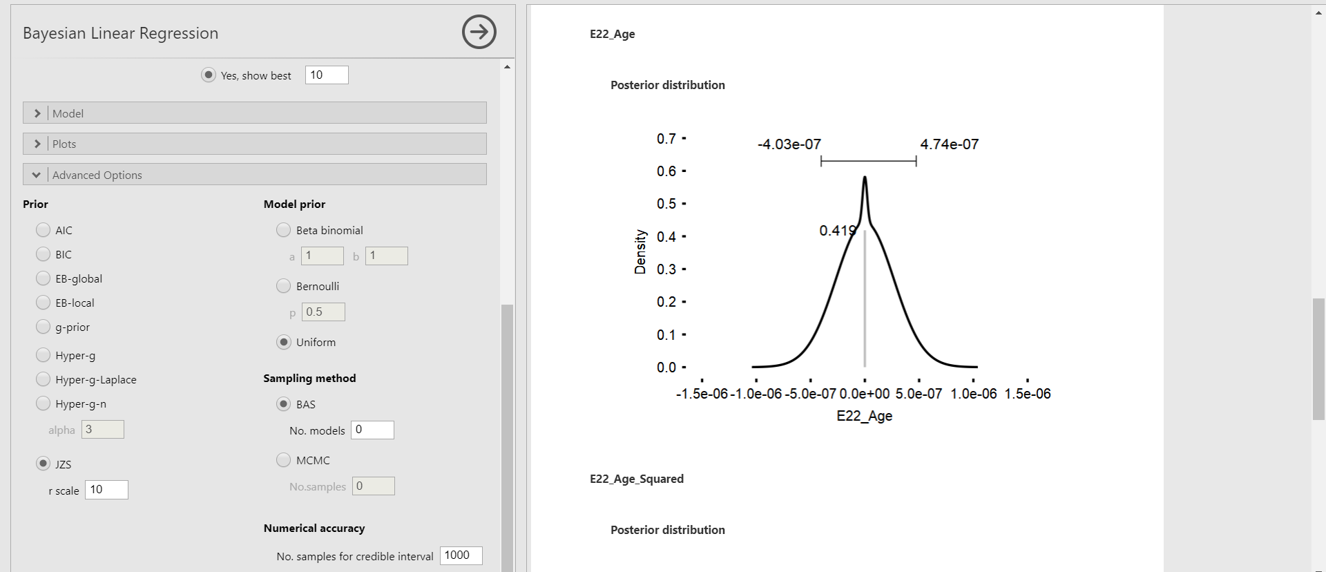
- With the marginal posterior distribution, we can see the posterior density of each parameter.
- Click Plots bar in the options panel -> Check Marginal posterior distributions under Coefficients
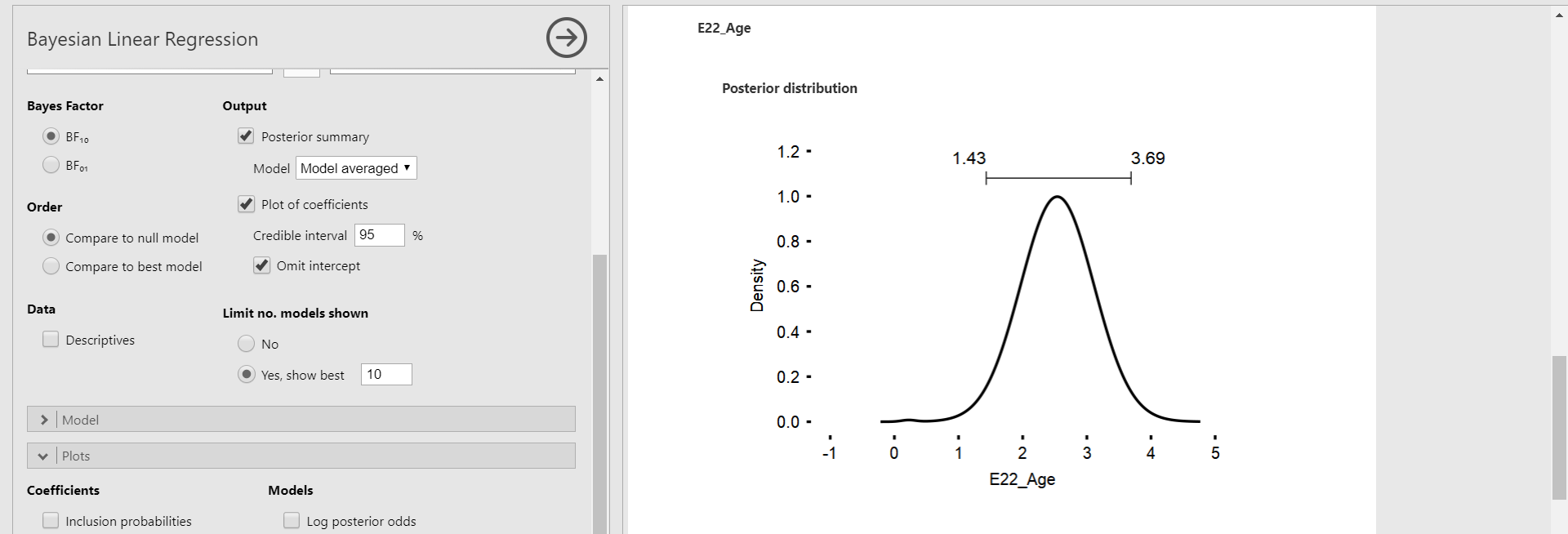

- We only focus on the marginal posterior distributions of age and age-squared variable, again. The bar above the highest peak corresponds to the 95% credible interval with the lower limit on the left and the upper limit on the right. This interval is the same as the 95% credible interval in the Posterior Summaries of Coefficients table.
3. So, tell me the default prior for the regression coefficients!
- Behind what we have been doing in interpreting the results, the default prior is hiding. To seek the default prior, click the Advanced Options bar in the options panel. The left column Prior presents the priors we can take.

- By default, The JZS prior with an r scale of 0.354 is chosen. The JZS prior stands for the Jeffreys-Zellner-Siow prior. It is the default prior that jamovi uses for Bayesian regression.
- Technically speaking, the JZS prior assigns the normal distribution to each regression coefficient (Andraszewicz et al., 2015). Of course, there are other options for prior choices such as AIC, BIC, EB-global, EB-local, g-prior, Hyper-g, Hyper-g-Laplace, and Hyper-g-n. The JZS prior, however, is most recommended and advocated as the default prior when performing Bayesian regression analysis. Thus, we proceed with adjusting the r scale values of the JZS prior. For readers who are interested in understanding the aforementioned priors, see Liang, Paulo, Molina, Clyde, and Berger (2008).
- Please note that under the Advanced Options bar, the Prior column on the left is about setting the prior distributions on the regression parameters whereas the Model prior column on the right is about assigning prior model probabilities.
V. Changing the r scale values of the JZS prior
- By setting different values of the r scale instead of 0.354, it is possible to change the scale or variance but not the location of the JZS prior. This idea is associated with what is called the prior sensitivity.
- You might be curious about how to incorporate prior knowledge by using different prior distributions and adjusting hyperparameters of them. Such functionality is currently not available in jamovi (jamovi version 1.2.27 & jsq version 1.0.1).
- The prior sensitivity, in a nutshell, tells us how robust the estimates are depending on the width of the prior distribution. Although we do not discuss the topic of prior sensitivity in detail, it is good to remember the key idea in case you encounter the concept in the Bayesian literature (for interested readers on the idea of prior sensitivity, see Van Erp, Mulder, and Oberski, 2018).
- In jamovi, changing the r scale values specifically indicates how certain we are about the null effects of parameters in the regression analysis. Larger values for the r scale correspond to wider priors whereas smaller values lead to the narrower priors.
- If a wider prior is adopted, hence more spread-out the prior distribution is, we are unsure about the effect of parameters. A narrower prior, on the other hand, means we have a strong belief that the effect is concentrated near zero (i.e., the null effect).
- The focus here is to compare the results of different r scale specifications (0.001, 0.1, 10, and 1000) of the JZS prior. Let’s see what happens in the parameter estimates and the inclusion Bayes factors of the Posterior Summaries of Coefficients table and the marginal posterior distributions.
- In the marginal posterior distributions, you will encounter the grey spike at zero with its height. The spike means the absence of the effect of the regression coefficient. The height indicates how much the data favors the exclusion of a specific predictor in the regression model after observing the data. This height is also called the posterior exclusion probability. If the posterior exclusion probability is high, this means that the observed data does not support to include the predictor.
1. Adjusting the r scale values (0.001, 0.1, 10, and 1000)
JZS prior with the r scale of 0.001


JZS prior with the r scale of 0.1


JZS prior with the r scale of 10


JZS prior with the r scale of 1000


Summary of the posterior mean and the posterior standard deviation
| \(Age\) | Default (JZS with r = 0.354) | JZS with r = 0.001 | JZS with r = 0.1 | JZS with r = 10 | JZS with r = 1000 |
|---|---|---|---|---|---|
| Posterior mean | 2.530 | 1.593 | 2.312 | 3.15e-13 | 0.00 |
| Posterior standard deviation | 0.590 | 0.930 | 0.566 | 2.02e-7 | 0.000 |
| \(Age^{2}\) | Default (JZS with r = 0.354) | JZS with r = 0.001 | JZS with r = 0.1 | JZS with r = 10 | JZS with r = 1000 |
|---|---|---|---|---|---|
| Posterior mean | -0.025 | -0.016 | -0.022 | -3.05e-15 | 0.00 |
| Posterior standard deviation | 0.006 | 0.009 | 0.006 | 2.11e-9 | 0.000 |
2. Effect of different prior specifications on parameter estimation
- Can we compare the results of parameter estimation over the different prior specifications? To examine whether the results are comparable with the analysis with the default prior, we check two things: the relative bias and the change of parameter estimates from the Posterior Summaries of Coefficients table.
Relative bias
- The relative bias is used to express the difference between the default prior and the user-specified prior.
- The formula for the relative bias follows: \(bias = 100*\frac{(model \; with \; specified \; priors\; – \; model \; with \; default \;priors)}{model \; with \; default \; priors}\)
- To preserve clarity, we will just calculate the bias of the two regression coefficients and only compare the model with the default prior (JZS prior with the r scale of 0.354) and the model with the different r scale value (JZS prior with the r scale of 0.001).
- For the age variable, the relative bias is \(100*\frac{(1.593\; – \; 2.530)}{2.530}\). This equals -37.04%.
- For the age-squared variable, the relative bias is \(100*\frac{(-0.016\; – \; (-0.025))}{-0.025}\), which equals -36%.
- We see that the influence of the user-specified prior is around -37% for the regression coefficient of the age variable and -36% for that of the age-squared variable. This is a sign of change in the results with different prior specifications. For the concrete examination, let’s take a look at the parameter estimates.
| \(Age\) | Default (JZS with r = 0.354) | User-specified (JZS with r = 0.001) |
|---|---|---|
| Posterior mean | 2.530 | 1.593 |
| Posterior standard deviation | 0.590 | 0.930 |
| 95% credible interval | [1.433, 3.690] | [-0.038, 2.83] |
| \(Age^{2}\) | Default (JZS with r = 0.354) | User-specified (JZS with r = 0.001) |
|---|---|---|
| Posterior mean | -0.025 | -0.016 |
| Posterior standard deviation | 0.006 | 0.009 |
| 95% credible interval | [-0.036, -0.013] | [-0.028, 3.35e-4] |
- For both variables, there are changes in the parameter estimates. Specifically, the 95% credible intervals with the default prior setting do not include 0. However, 0 is included in the 95% credible intervals when the user-specified prior is used. Therefore, there is no evidence of the effect of regression coefficients when we use the prior with the r scale of 0.001. These results are understandable since we set the very small r scale value (0.001), which indicates our strong belief that there is no effect of predictors.
3. Effect of different prior specifications on inclusion Bayes factor
- This time, let’s take a look at how the inclusion Bayes factor changes over the different prior specifications. We check the relative bias and the change of inclusion Bayes factors from the Posterior Summaries of Coefficients table.
Relative bias
- We compute the relative bias of the inclusion Bayes factors of the two regression coefficients and only compare the model with the default prior (JZS prior with the r scale of 0.354) and the model with the different r scale value (JZS prior with the r scale of 0.001).
- For the age variable, the relative bias is \(100*\frac{(6.33\; – \; 464.54)}{464.54}\). This equals -98.64%.
- For the age-squared variable, the relative bias is \(100*\frac{(6.21\; – \; 312.75)}{312.75}\), which equals -98.01%.
- We see that the influence of the different prior specifications is around -98% for both inclusion Bayes factors. This is a sign of a large change in the results with different prior specifications. For a concrete examination, let’s look at the values of the inclusion Bayes factor.
| \(Age\) | Default (JZS with r = 0.354) | User-specified (JZS with r = 0.001) |
|---|---|---|
| \(BF_{inclusion}\) | 464.54 | 6.33 |
| \(Age^{2}\) | Default (JZS with r = 0.354) | User-specified (JZS with r = 0.001) |
|---|---|---|
| \(BF_{inclusion}\) | 312.75 | 6.21 |
- For both variables, the inclusion Bayes factors with the r scale of 0.001 are much smaller than those with the default prior. This happened since a strong belief about the null effect of the regression coefficients is reflected in the smaller r scale value.
4. Conclusion about the effect of different prior specifications
- Given the relative bias, parameter estimates, and the inclusion Bayes factors, we conclude there exists a difference from different prior specifications. We thus would not end up with similar conclusions.
- The influence of prior also depends on the size of the dataset. The sample size for our data is 333, which is relatively big. In the case of the big dataset, the influence of the prior is relatively small. If one would use a smaller dataset, on the other hand, the influence of the prior becomes larger.
VI. Epilogue
- Congratulations! You are standing at the ending point. Some parts might be tricky, but we hope you found it useful and informative.
- We wish this tutorial can benefit a lot of applied researchers who use jamovi for performing Bayesian regression analyses!
References
Andraszewicz, S., Scheibehenne, B., Rieskamp, J., Grasman, R., Verhagen, J., & Wagenmakers, E. J. (2015). An introduction to Bayesian hypothesis testing for management research. Journal of Management, 41(2), 521-543. https://doi.org/10.1177/0149206314560412
Hinne, M., Gronau, Q. F., van den Bergh, D., & Wagenmakers, E. J. (2020). A conceptual introduction to Bayesian model averaging. Advances in Methods and Practices in Psychological Science, 3(2), 200-215. https://doi.org/10.1177/2515245919898657
Hoeting, J. A., Madigan, D., Raftery, A. E., & Volinsky, C. T. (1999). Bayesian model averaging: a tutorial. Statistical science, 382-401.
Kass, R. E., & Raftery, A. E. (1995). Bayes factors. Journal of the American Statistical Association, 90(430), 773-795.
Kruschke, J. (2014). Doing Bayesian Data Analysis: A Tutorial with R, JAGS, and Stan (2nd ed.). Academic Press.
Liang, F., Paulo, R., Molina, G., Clyde, M. A., & Berger, J. O. (2008). Mixtures of g priors for Bayesian variable selection. Journal of the American Statistical Association, 103(481), 410-423. https://doi.org/10.1198/016214507000001337
The jamovi project. (2020). jamovi (Version 1.2.27)[Computer software].
Van de Schoot, R. (2020). PhD-delay Dataset for Online Stats Training [Data set]. Zenodo. https://doi.org/10.5281/zenodo.3999424
Van de Schoot, R., Kaplan, D., Denissen, J., Asendorpf, J. B., Neyer, F. J., & Van Aken, M. A. (2014). A gentle introduction to Bayesian analysis: Applications to developmental research. Child development, 85(3), 842-860. https://doi.org/10.1111/cdev.12169
Van de Schoot, R., Yerkes, M. A., Mouw, J. M., & Sonneveld, H. (2013). What took them so long? Explaining PhD delays among doctoral candidates. PloS one, 8(7), e68839. https://doi.org/10.1371/journal.pone.0068839
Van den Bergh, D., Clyde, M. A., Raj, A., de Jong, T., Gronau, Q. F., Marsman, M., Ly, A., & Wagenmakers, E. J. (2020). A Tutorial on Bayesian Multi-Model Linear Regression with BAS and JASP. https://doi.org/10.31234/osf.io/pqju6
Van Erp, S., Mulder, J., & Oberski, D. L. (2018). Prior sensitivity analysis in default Bayesian structural equation modeling. Psychological Methods, 23(2), 363-388. https://doi.org/10.1037/met0000162