jamovi for beginners
Ihnwhi Heo and Rens van de Schoot
Department of Methodology and Statistics, Utrecht University
Last modified: 02 November 2020
This tutorial introduces the basics of jamovi (The jamovi project, 2020) for beginners. Starting from jamovi installation, we explain the screen structure of jamovi, how to load a dataset, and how to explore and visualize data. Readers will further learn ways to perform such statistical analyses as correlation analysis, multiple linear regression, t-test, and one-way analysis of variance, all from a frequentist viewpoint. Given the integrative power between jamovi and R, one section is designed to help readers to make use of the best of both jamovi and R. After the tutorial, we expect readers to become familiar with using basic options in jamovi and get prepared for the ‘next step’.
Since we continuously improve the tutorials, let us know if you discover mistakes, or if you have additional resources we can refer to. If you want to be the first to be informed about updates, follow Rens on Twitter.
How to cite this tutorial in APA style
Heo, I., & Van de Schoot, R. (2020, November). Tutorial: jamovi for beginners. Zenodo. https://doi.org/10.5281/zenodo.4008373
Popularity Dataset
We will use a popularity dataset (Van de Schoot, 2020) from Van de Schoot, Van der Velden, Boom, and Brugman (2010). To download the dataset, click here.
The dataset is based on a study that investigates an association between popularity status and antisocial behavior from at-risk adolescents (n = 1,491), where gender and ethnic background are moderators under the association. The study distinguished subgroups within the popular status group in terms of overt and covert antisocial behavior.
For more information on the sample, instruments, methodology, and research context, we refer the interested readers to the paper (see references). A brief description of the variables in the dataset follows. The variable names in the table below will be used in the tutorial, henceforth.
| Variable name | Description |
|---|---|
| respnr | Respondents’ number |
| Dutch | Respondents’ ethnic background (0 = Dutch origin, 1 = non-Dutch origin) |
| gender | Respondents’ gender (0 = boys, 1 = girls) |
| sd | Adolescents’ socially desirable answering patterns |
| covert | Covert antisocial behavior |
| overt | Overt antisocial behavior |
How to cite the dataset in APA style
Van de Schoot, R. (2020). Popularity Dataset for Online Stats Training [Data set]. Zenodo. https://doi.org/10.5281/zenodo.3962123
I. Ice-breaking with jamovi
1. What makes jamovi attractive?
- Free, open-source, and simple to use statistical software
- Integration with R
- A user guide and community resources from the jamovi website
2. Download jamovi and seat it on your computer
- Let’s head for this website.
- Irrespective of your operating systems, there are two options for downloading: solid and current.
- The solid release is tested several times for stable and reliable use of jamovi. The current release, on the other hand, contains new features following the recent development, so it might contain minor bugs. We download the solid release for the current tutorial.
- Think about what your operating system is.
- If you use Windows, find the OS column under the ‘All Releases’ section -> Click
Windows solid .exe with the latest.version.number - If you use Mac, find the OS column under the ‘All Releases’ section -> Click
macOS solid .dmg with the latest.version.number - If you use Linux, find the OS column under the ‘All Releases’ section -> Click
Linux flathub with the latest.version.number-> ClickINSTALL - If you use ChromeOS, find the OS column under the ‘All Releases’ section -> Click
ChromeOS flathub with the latest.version.number-> ClickINSTALL
- If you use Windows, find the OS column under the ‘All Releases’ section -> Click
3. How jamovi’s screen looks like
- Open the jamovi and see how it looks like. Do you encounter a snapshot below?
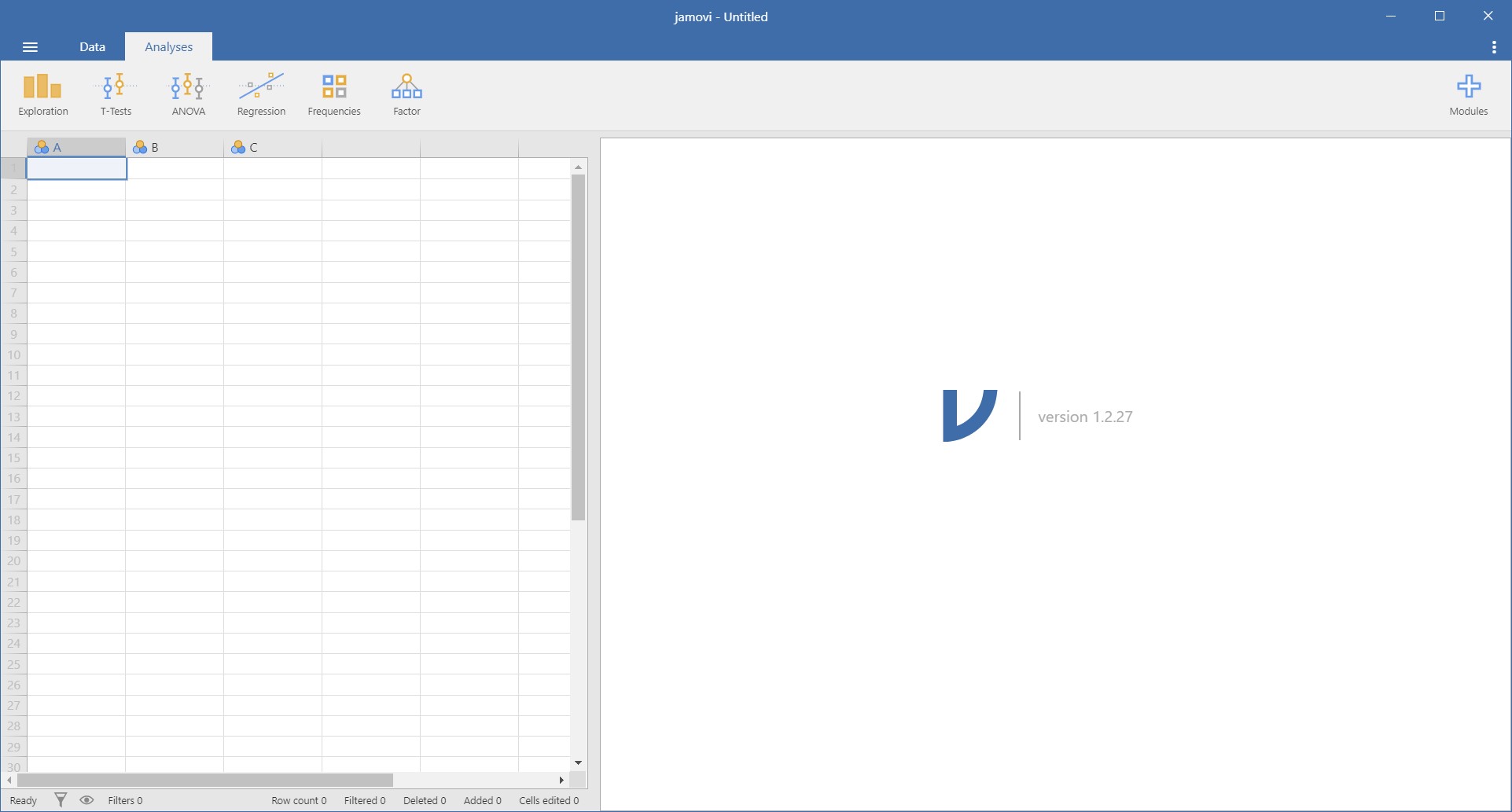
- Let’s divide the jamovi screen structure into two parts to illustrate their respective roles.
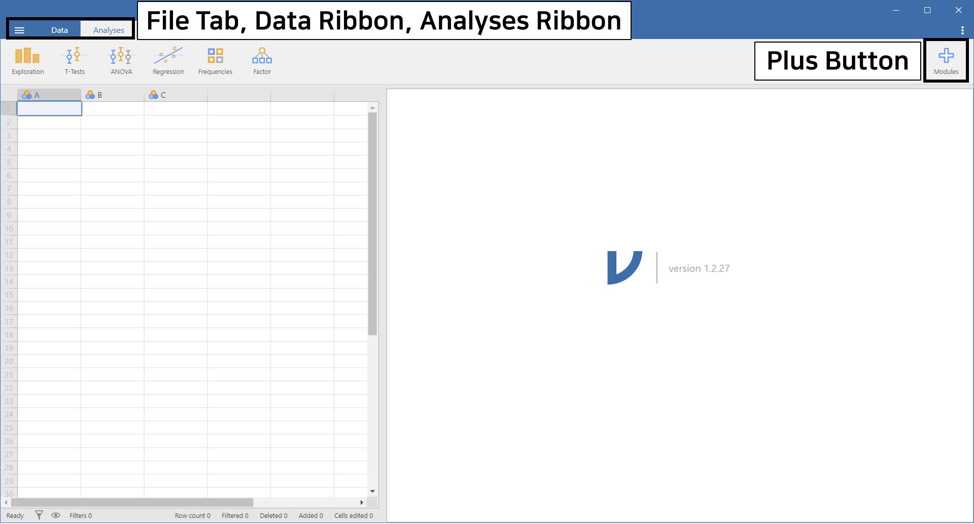
File Tab, Data Ribbon, and Analyses Ribbon

- From left to right, there are three options: file tab, data ribbon, and analyses ribbon. Let’s click each option and figure out how they help us.
- First, click the leftmost file tab, which is a layer with three horizontal levels. We highlighted the file tab within the black solid box in the above picture.
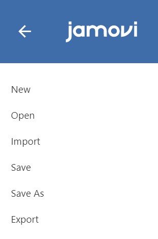
- We see six commands appear. With the file tab, you can open, save, or export what you performed in jamovi.
- This time, we will click the data ribbon (again emphasized in the solid rectangle). Simultaneously focus on which buttons appear when you click the data ribbon.
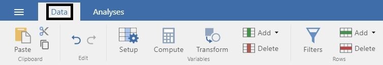
- Data ribbon concerns with managing data, in general. If you want to add a new column, compute a new variable, filter certain values of a variable, and so on, find the data ribbon!
- What’s remaining? Analyses ribbon! Click the rightmost analyses ribbon (yes, emphasized in the solid-line box). Don’t forget to enjoy looking at which buttons appear.

- We can see such buttons as Exploration, T-Tests, ANOVA, and more. As the name ‘Analyses’ implies, the analyses ribbon helps explore loaded data and perform various statistical analyses. For example, if you want to perform regression analysis, simply click the ‘Regression’ button. Shall we try?
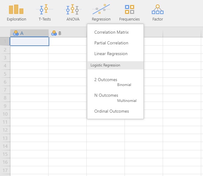
- Six options for regression analysis appear.
- “Oh, looks cool! It seems like those are the only things I can do, though.” Never! Depending on your needs, jamovi helps you perform advanced analyses. How to? See the plus button below.
Plus button

- As the plus sign implies, the plus button is meant to be the add-on module button for advanced analytic options. Let’s click the plus button to take a look at what it does.
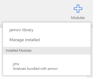
- There are options like jamovi library, Manage installed, Installed Modules, and jmv.
- In jamovi, statistical analyses beyond the provided options can be implemented by installing modules. To install modules, we visit the jamovi library (not to borrow books!). Note that this library is ever developing, and even ‘you’ can open your library. If you are an R user, this system is quite familiar with CRAN and what R function
install.packages()does. - By default, the jmv module is installed. You can check the list of installed modules under the installed Modules header. This jmv module contains basic and some advanced statistical analyses under the analyses ribbon.
- One more option to go: Manage installed. We have an intuition that it may have something to do with managing installed modules including removing modules. This is exactly what the Mange installed option does.
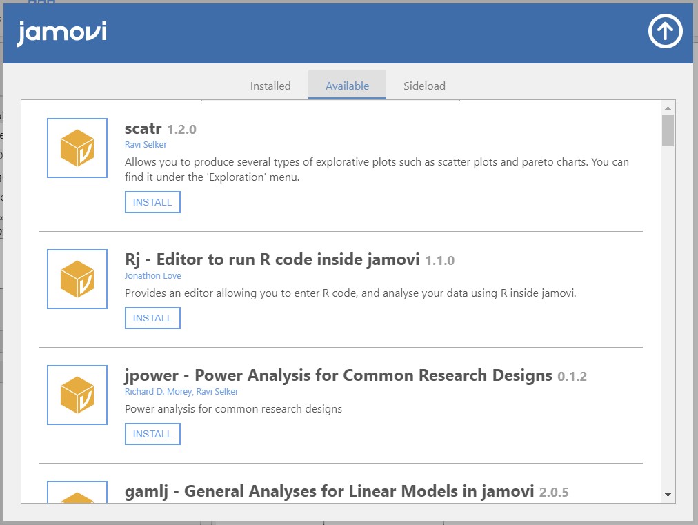
- Okay, now it is a good time to enjoy the showcases of jamovi modules. Click the jamovi library.
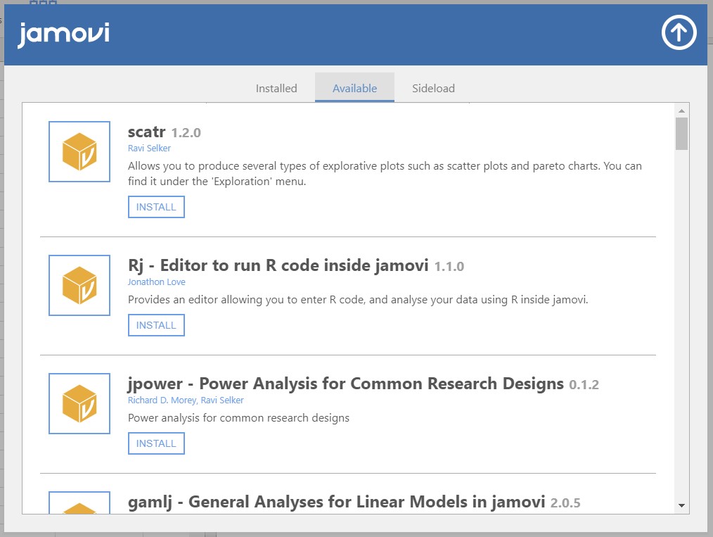
- We can see such modules as scatr, Rj, jpower, gamlj, and much more if we scroll down. These are all modules that can be installed on jamovi. The extensive list of jamovi modules is also available here.
- As a practice, let’s download one certain module for Bayesian statistical analyses. We do not deal with the Bayesian statistics in the current tutorial, but it is necessary for our ‘next step’! To download the module, scroll down, and find the module called jsq – Bayesian Methods.
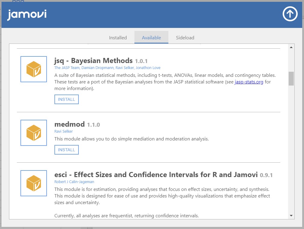
- Click INSTALL to add the jsq – Bayesian Methods module on jamovi.
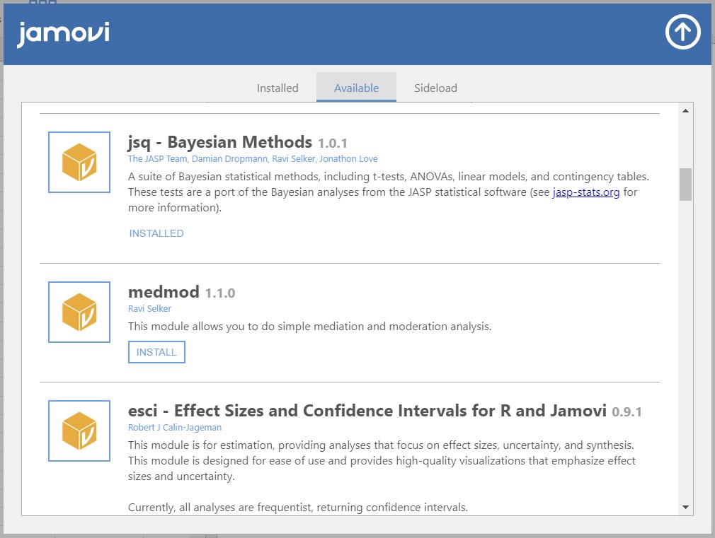
- Once the installation is done, the INSTALL button has been changed into INSTALLED.
- Click the upper-headed arrow on the top right of the pop-up to go back to the main screen of jamovi. Next, click the plus button, again.
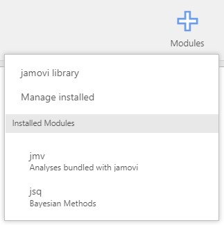
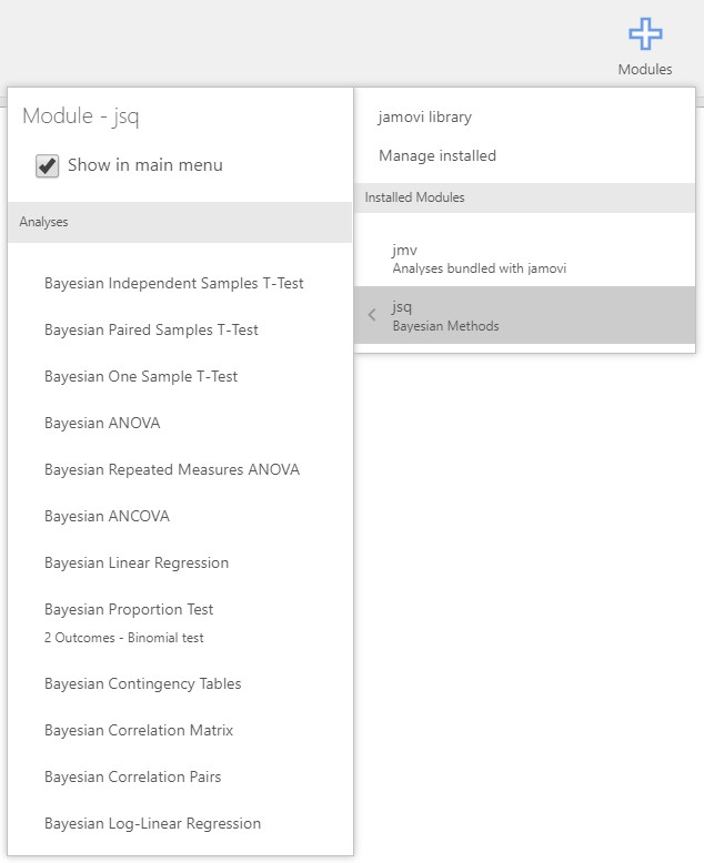
- Under the Installed Modules header, the jsq module has been added. If you move your mouse cursor on jsq, a list of Bayesian analytic options appears.
- We can also see these options if we click the analyses ribbon. Really? Let’s click the Regression button under the analyses ribbon.
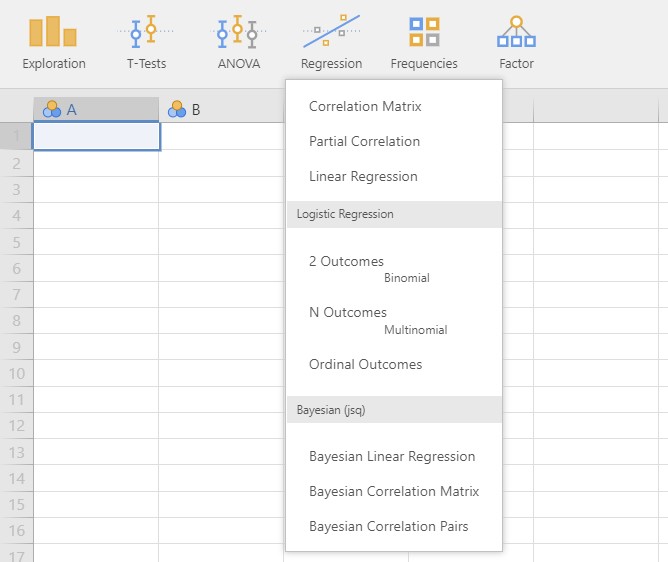
- There indeed exist three additional choices for performing Bayesian regression, compared to what we saw previously. Before we download the jsq module, these Bayesian regression options did not exist.
- Where should we go if we are to remove the jsq option? Click the plus button and go to Manage installed!
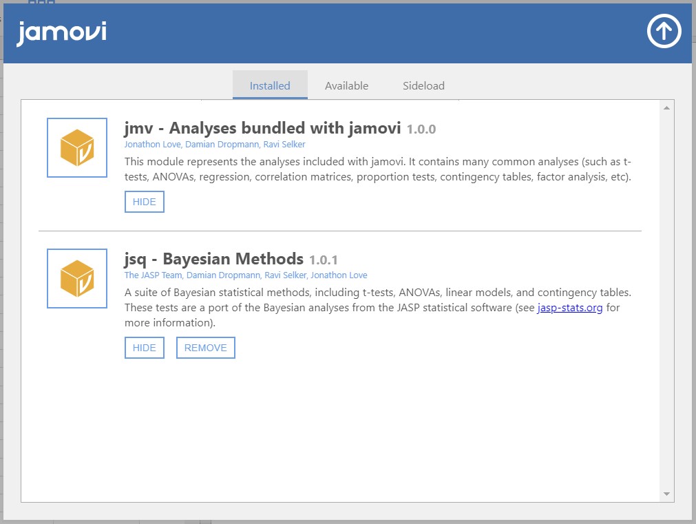
- We see there are currently two modules installed on jamovi. You can anytime delete the installed modules by clicking REMOVE.
II. Prepare your data on jamovi
- A prerequisite for statistical analysis is a dataset, needless to say. You can easily load the data with several mouse clicks. Can you guess which button should we use to do this? Yes, the file tab!
- jamovi offers two ways to load the data. One is from your computer and the other is from the in-built data library.
- To download the dataset that we will use (
popular_regr_1), click here.
1. From your computer
- Click file tab -> Open -> This PC -> Browse -> Open your file
- This is all you need to do. How easy! Can you see the loaded dataset or the spreadsheet as the picture below?
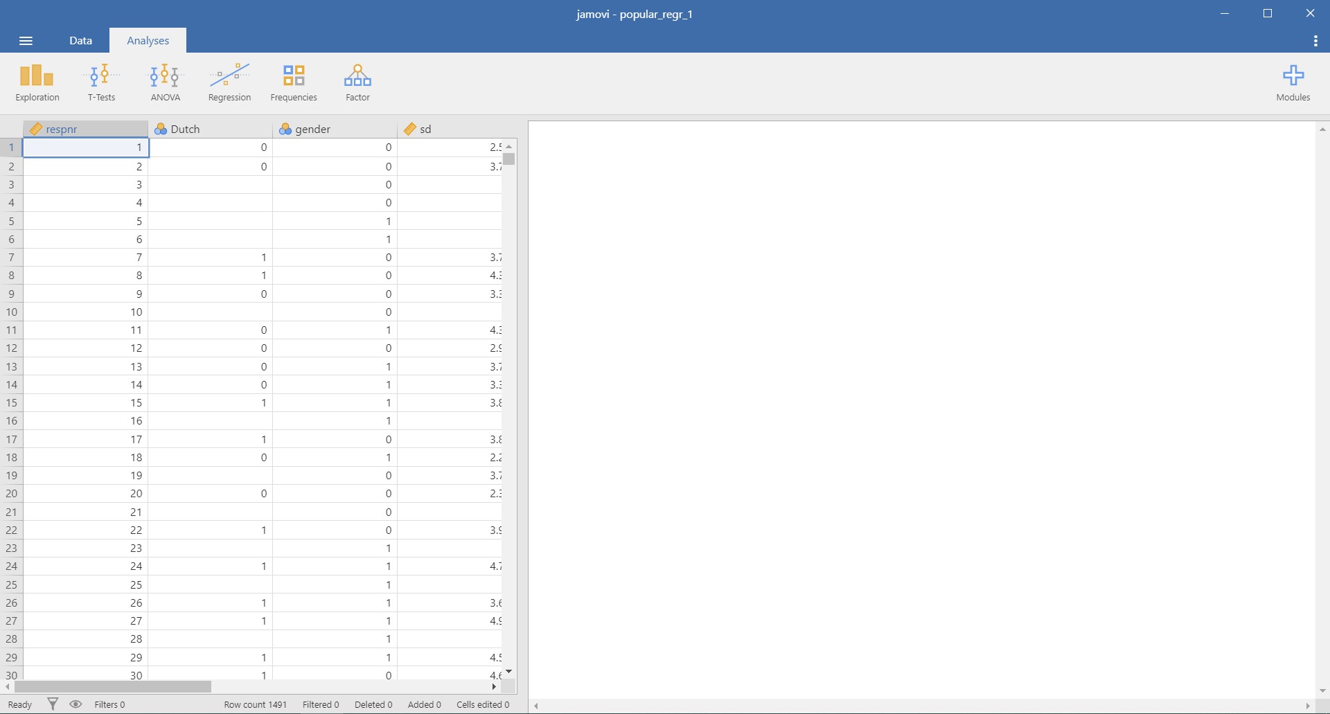
- There is one advantage in jamovi after loading the data. Imagine you are skimming through the spreadsheet to check whether all entries are correct. All of a sudden, you detect that some data entries are wrong, so you need to fix certain values.
- If that happens, you can simply go to the spreadsheet and modify values directly. This is similar to what we can do in Microsoft Excel! You may also find it useful to use buttons under the data ribbon. So, without switching multiple screens, you can load and edit the data entries simultaneously.
2. From the data library
- Note that jamovi (in version 1.2.27) offers four in-built datasets. First three of them are example datasets of correlation, ANOVA, and repeated measures ANOVA, respectively. The fourth one is the iris data (Anderson, 1936) popularly used for machine learning.
- Assuming that we are interested in performing correlation analysis (what we are going to do, soon!), let’s load the Big 5 personality dataset (Dolan, Oort, Stoel, & Wicherts, 2009).
- Click file tab -> Open -> Data Library -> Click Big 5
III. Exploring data
1. Understanding the data numerically
Descriptive statistics
- If you are keen on knowing the mean, the median, the maximum value, and more about the variables in your data, you should take a look at the descriptive statistics. Let’s examine the descriptive statistics of the variables in the
popular_regr_1dataset. - Go to the analyses ribbon -> Exploration -> Descriptives -> Move the six variables to the Variables section on the right. To do that, select all the variables and click the right-headed triangle button. You can also drag these variables to the Variables section.
- “I see some symbols left to the variable names. What are they?” A nice catch! Those symbols indicate the measurement level of the corresponding variables. For instance, a symbol that looks like a ruler refers to a scale variable (also called a continuous variable). A symbol with three colorful circles indicates a nominal variable. If you have experience in using SPSS, you can catch that those symbols are identical to those in SPSS.
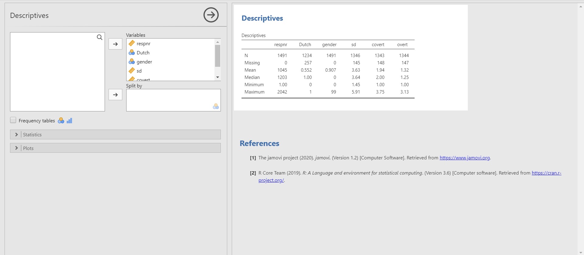
- After you move the variables, jamovi immediately prints the output on the right section of the screen.
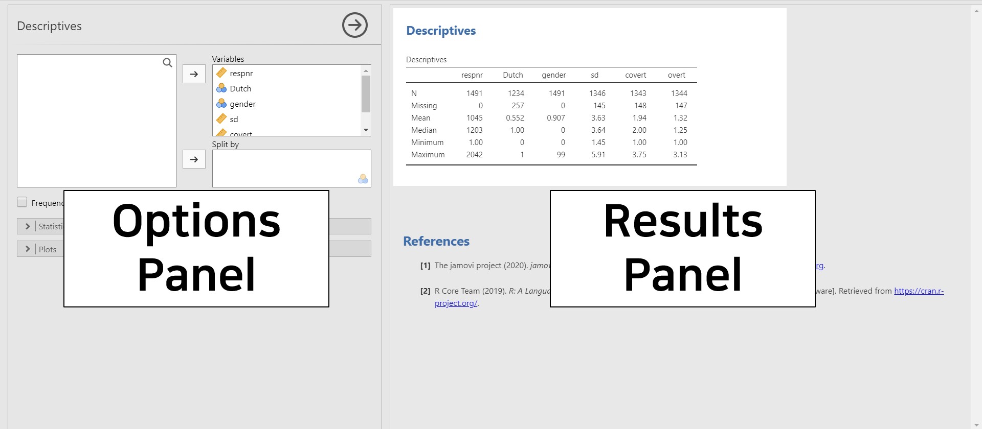
- For convenience, let’s refer to a left panel as an options panel and a right panel as a results panel.
- Take a look at the results panel (right panel). You can see the table with descriptive statistics. The first column of the table presents six pieces of information about the variable. N is the sample size excluding the missing values. For the variable overt, there are 1344 entries. The number of missing values, on the other hand, is presented in the Missing row. For overt, there are 147 missing values. Consequently, the sum between N and Missing equals the total sample size for each variable. For overt, there are 1491 samples (the sum between 1344 and 147 is 1491). The mean and the median of overt are 1.32 and 1.25. The maximum and minimum of overt are 1 and 3.13.
- What if we want to check more descriptive statistics including the standard deviation, the mode, the range, the skewness? Look at the options panel (left panel). What you need to do is to click the Statistics bar. Next, check Std. deviation and Range under Dispersion, check Mode under Central Tendency, and Skewness under Distribution.
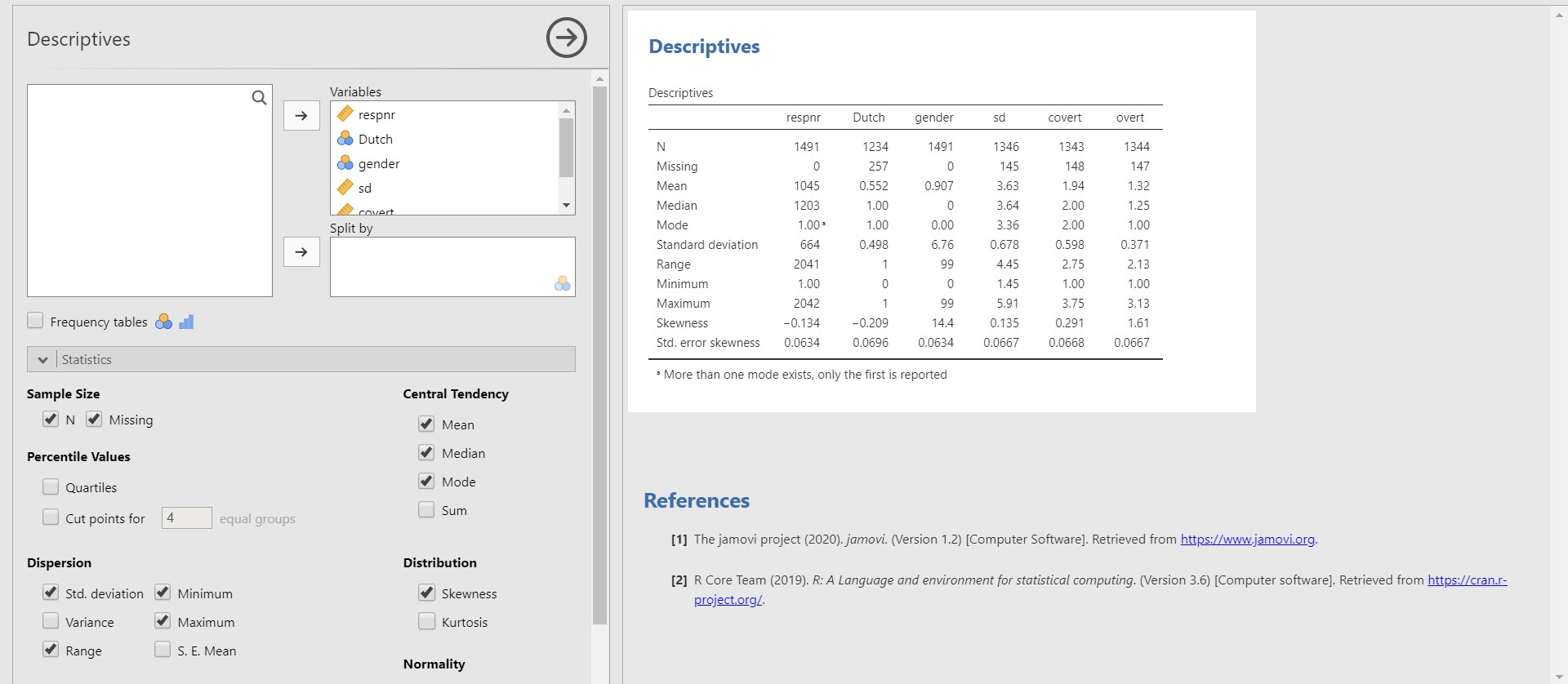
- Now jamovi gives additional descriptive statistics we wanted to see. For instance, the standard deviation and the range of overt are 0.371 and 2.13.
Frequency tables
- In case there are categorical variables (nominal and ordinal variables), frequency tables show the frequency of each category (a category is also referred to as a level in statistics).
- Check Frequency tables in the options panel. The checkbox of Frequency table is located above the Statistics bar.
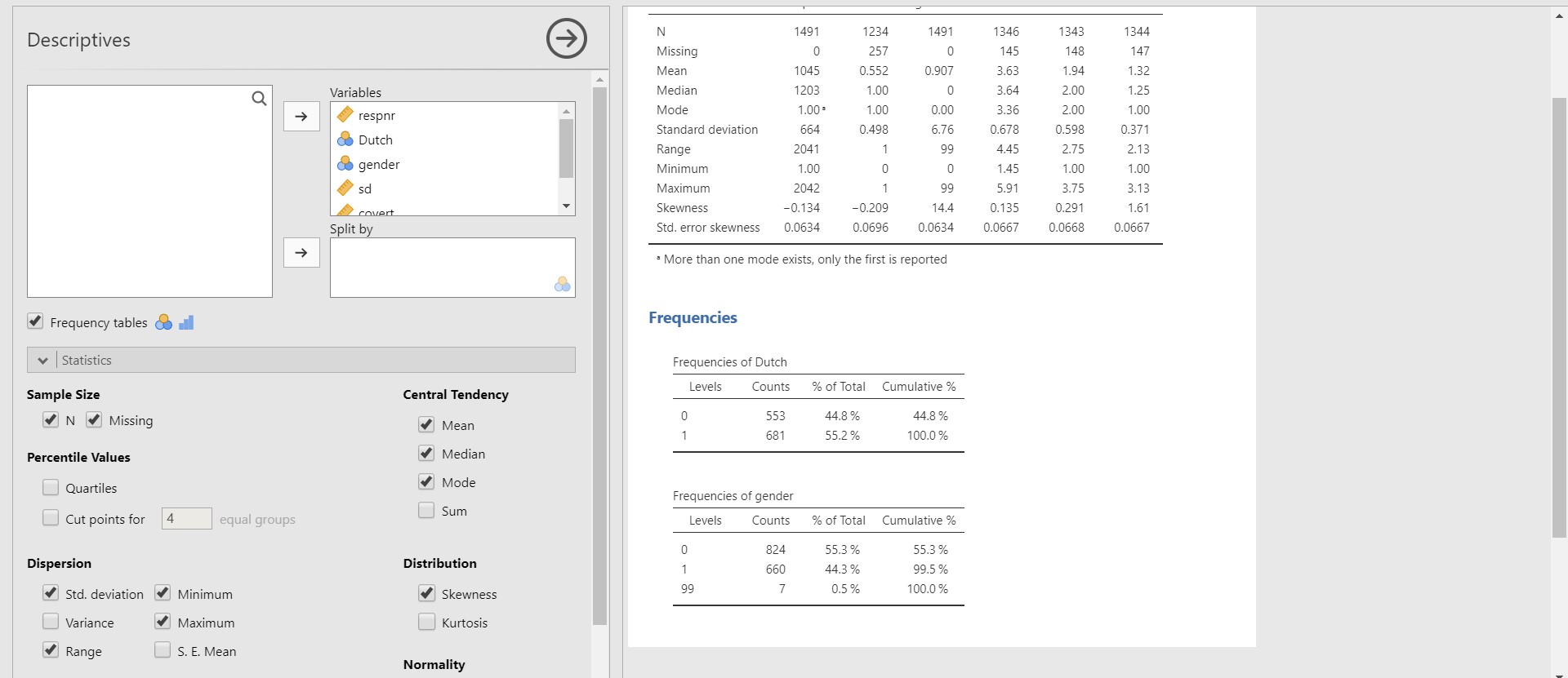
- Since there are two categorical variables, Dutch and gender, two frequency tables are presented. For example, look at the frequency table for Dutch. There are 553 cases coded as 0 (Dutch origin) and 681 coded as 1 (non-Dutch origin).
2. Understanding the data visually
- In doing statistics, images are oftentimes efficient tools to convey information than numbers. Think about the skewness of the variable. Rather than a number, looking at the distribution is more intuitive.
- We keep going a visual investigation of variables while putting all six variables under the Variables section.
Histogram
- If you are curious about how the values of one variable are distributed, drawing a histogram is one way of doing that.
- Click Plots bar in the options panel -> Check Histogram
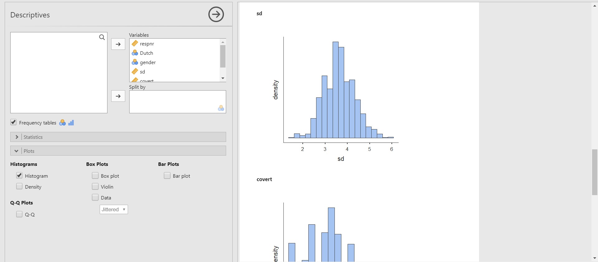
- On the results panel, jamovi produces a histogram for socially desirable answering patterns (sd), for example.
Boxplot
- A great way to investigate the dispersion of the data from the median and checking the existence of outliers is to draw a boxplot.
- Click Plots bar in the options panel -> Check Box plot
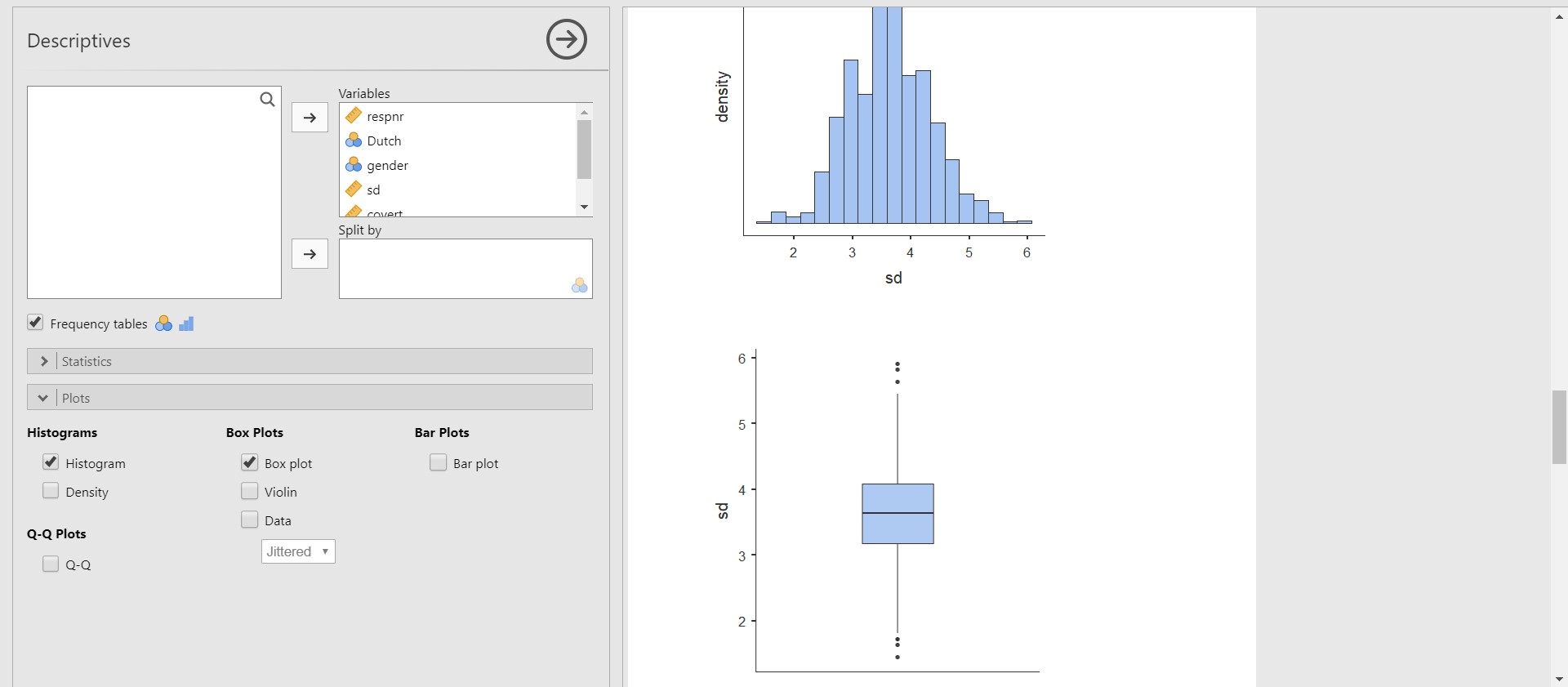
- Please note that the boxplots of each variable are plotted below the histograms of the corresponding variables. Take a look at the boxplot of the sd (socially desirable answering patterns). We can detect that outliers exist.
Scatter plot
- Scatter plots are what you can choose when describing the relationship between two variables.
- To draw a scatter plot, we need to install a new module. So, it is a great time to recapitulate what we have learned about adding modules!
- Click the plus button on the top right of the jamovi screen -> Click jamovi library -> Find scatr module (in jamovi version 1.2.27, the scatr module is the first on the list!)
- Press INSTALL -> Click the upper-heading arrow on the top right of the pop-up to hide the library
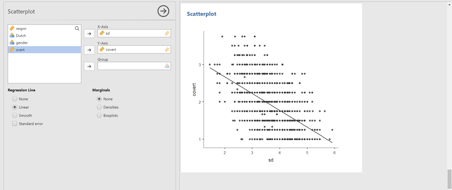
- Click the analyses ribbon -> Click Exploration -> Scatterplot
- For illustrative purposes, let’s visualize the relationship between socially desirable answering patterns (sd) and covert antisocial behavior (covert).
- Move sd to the X-Axis section and covert to the Y-Axis section.
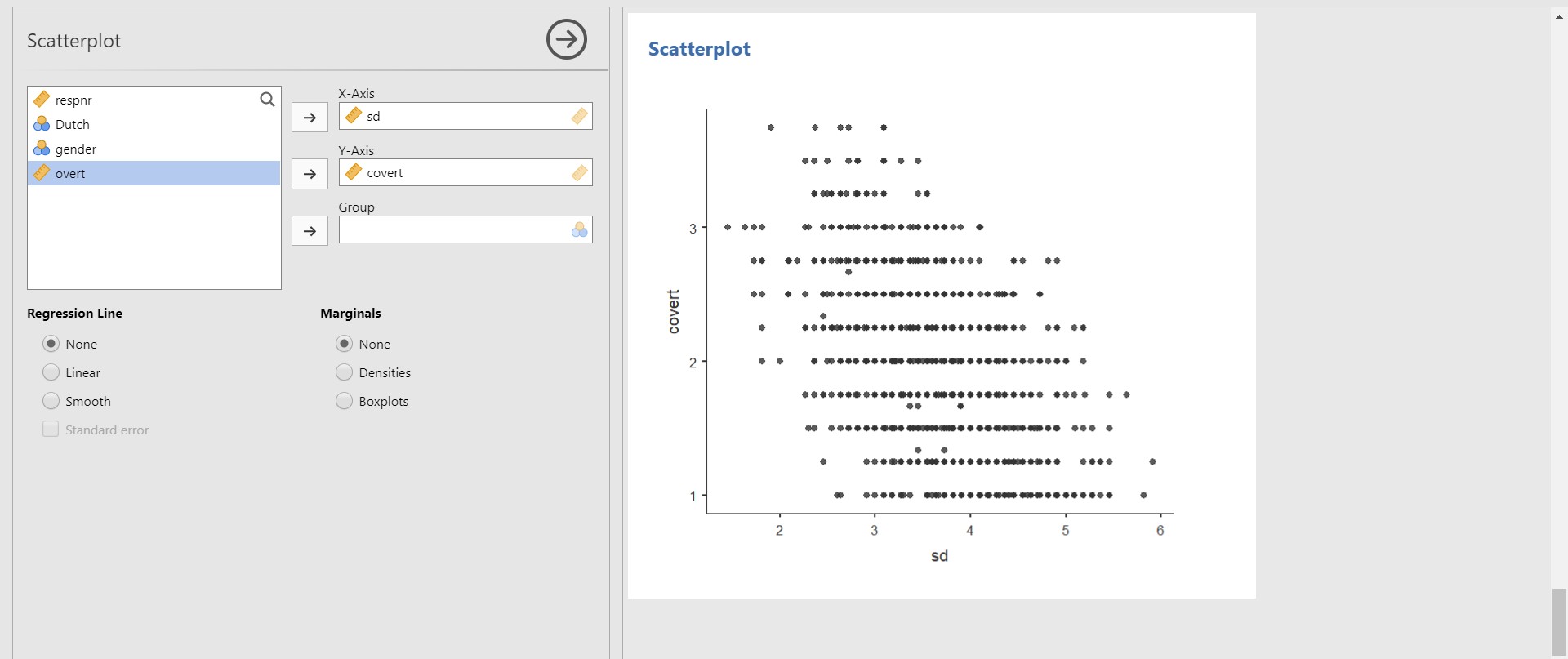
- Given the scatter plot, it seems like there exists a negative correlation between socially desirable answering patterns (sd) and covert antisocial behavior (covert). In other words, the more covert antisocial behavior is, the less socially desirable answering patterns are. To be certain about this observed pattern, you can draw a regression line. Under Regression Line, check Linear.
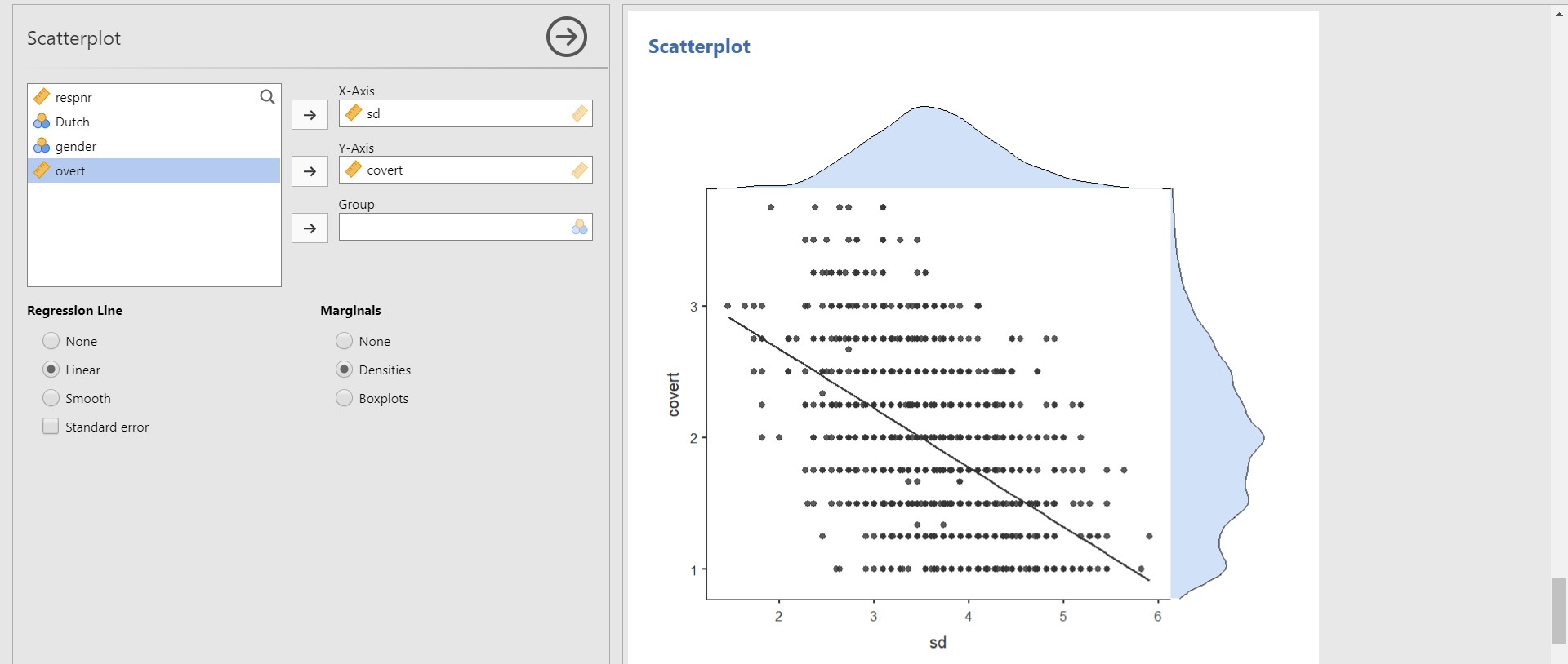
- You can also add either densities or boxplots of variables on the plot margins. All you need to do is to check Densities under Marginals if you are interested in the densities of each variable. Then, the density of the sd (x-axis) will be plotted at the top of the scatter plot whereas that of the covert (y-axis) on the right side of the scatter plot.
IV. Analysis and interpretation of data
- In this tutorial, we fully focus on basic statistical analysis in the frequentist statistics framework. However, it does not mean that we will never deal with Bayesian stuff. In ‘VI. Epilogue’, we guide you to another tutorial that illustrates how to conduct Bayesian statistics in jamovi. This is the reason why we installed the jsq module before (yes, our next step is doing Bayesian statistics)!
- At this point, readers might be curious about what exactly the Bayesian statistics is, what the differences are compared to frequentist statistics, and how it helps substantive researchers to answer research questions. For interested readers, we refer to two great easily-written papers!
- A gentle introduction to Bayesian analysis: Applications to developmental research (Van de Schoot, Kaplan, Denissen, Asendorpf, Neyer, & Van Aken, 2014)
- Bayesian analyses: Where to start and what to report (Van de Schoot & Depaoli, 2014)
- We assume that all the assumptions required for subsequent analyses are satisfied.
1. Correlation analysis
- To test if the correlation coefficient between two variables is significantly different from 0, we should conduct a correlation analysis.
- Go to the analyses ribbon -> Click Regression -> Correlation Matrix -> Choose at least two variables
- Let’s run the correlation analysis to examine whether the correlation coefficient between the covert and overt antisocial behavior (covert and overt) is significantly different from 0.
- From now on, we will use the alpha level of .05 because it is most commonly used.
- To do so, move the two variables, overt and covert, to the right section.
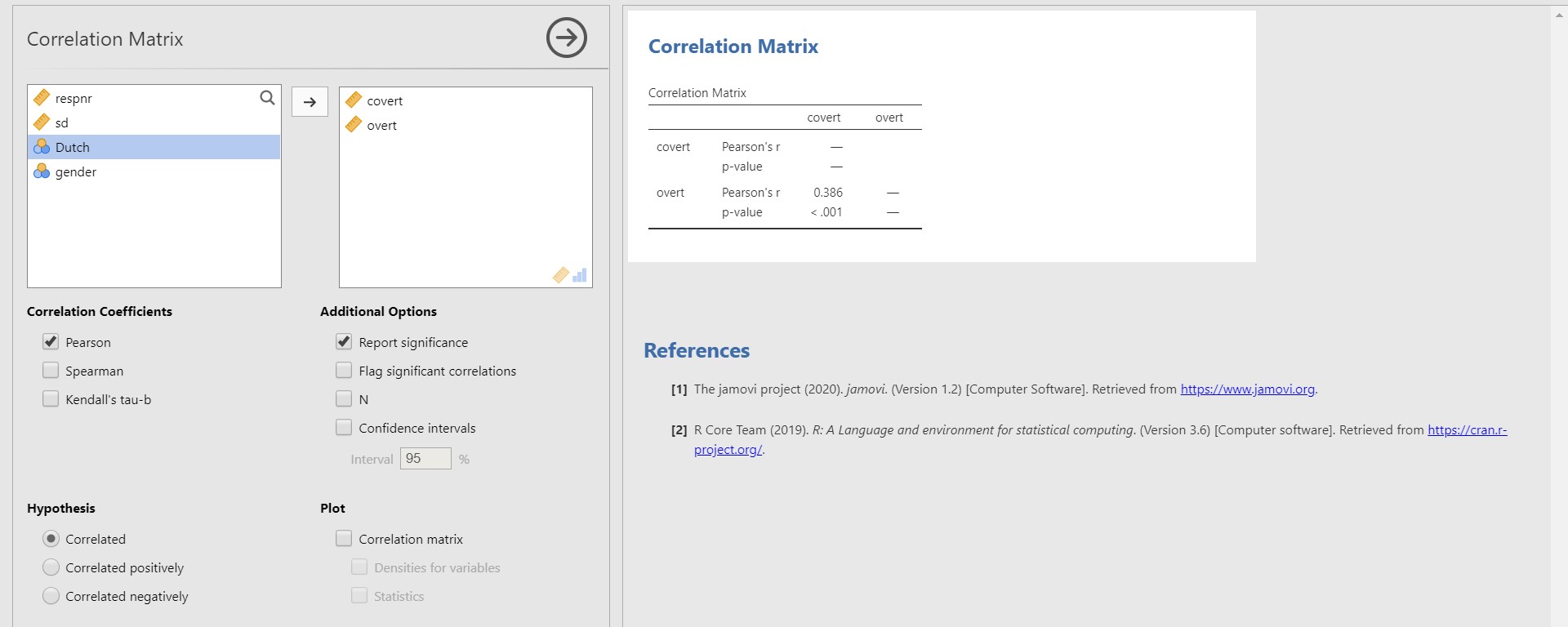
- According to the correlation matrix in the results panel, the correlation coefficient between covert and overt is 0.386, and the p-value is lower than 0.001. Therefore, the correlation coefficient of 0.386 is significantly different from 0.
2. Multiple linear regression
- When you are keen on predicting outcomes of a continuous dependent variable with multiple continuous or categorical independent variables, multiple linear regression analysis is performed.
- Go to the analyses ribbon -> Click Regression -> Linear Regression -> Choose one variable for Dependent Variable and other variables for Covariates (Covariates refer to independent variables)
- For illustrative purposes, let’s try to predict adolescents’ socially desirable answering patterns (sd) with overt and covert antisocial behavior (overt and covert). Accordingly, we should use sd as the dependent variable and overt and covert as the independent variables. Move sd under the Dependent Variable section and covert and overt under the Covariates section.
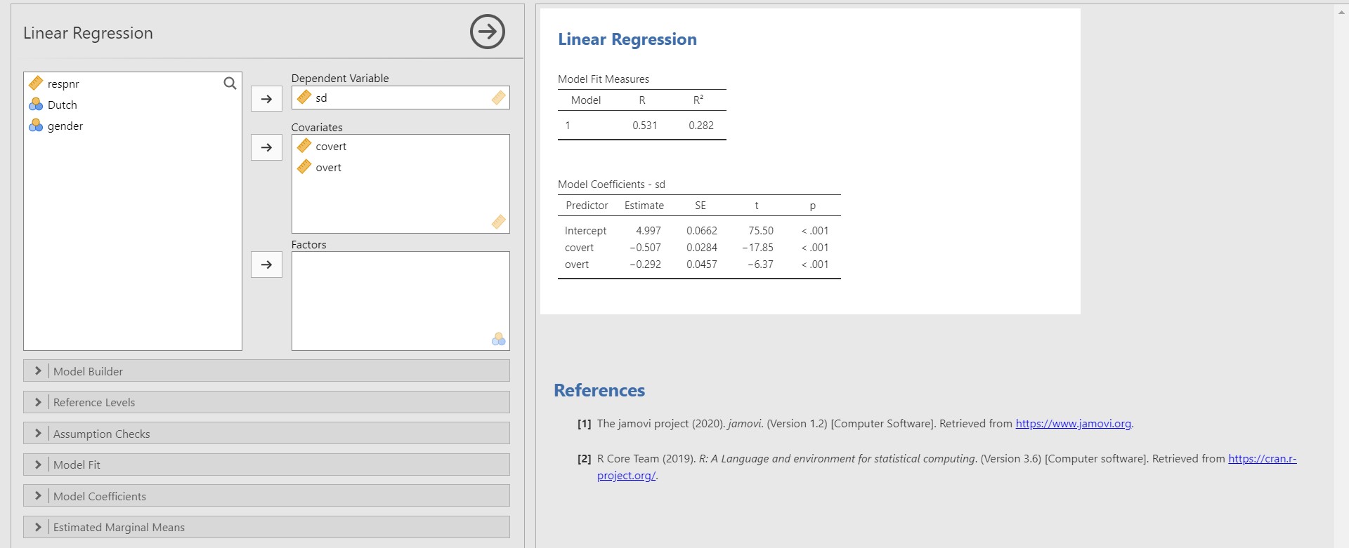
- First, look at the table under Model Coefficients – sd in the results panel.
- The unstandardized regression coefficient of covert is -0.507, and the p-value is lower than 0.001. You can find this value at the cross-section between the covert row and the Estimate column. This result means that the variable, covert, is a significant predictor with an alpha level of .05. If one unit of covert increases, the sd decreases 0.507 units.
- The unstandardized regression coefficient of overt is -0.292 with the p-value lower than 0.001. Therefore, the variable, overt, is a significant predictor of sd with an alpha level of .05. If one unit of overt increases, the sd decreases 0.292 units.
- Second, let’s look at the R-squared, which is indicated in the table under Model Fit Measures (note that our model is denoted as number 1). The R-squared is the proportion of variance explained by predictors. Therefore, the R-squared value of 0.282 means that the two predictors, covert and overt, explain 28% of the variance of sd.
- “Well… I am interested in getting more information like standardized regression coefficients or F-test. Where can I find them?” A great question! If that is the case, we have to ask jamovi to present us with those outputs via the options panel.
- For the standardized regression coefficients, check Standardized estimate under the Model Coefficients bar. For the F test, check F test under the Model Fit bar.
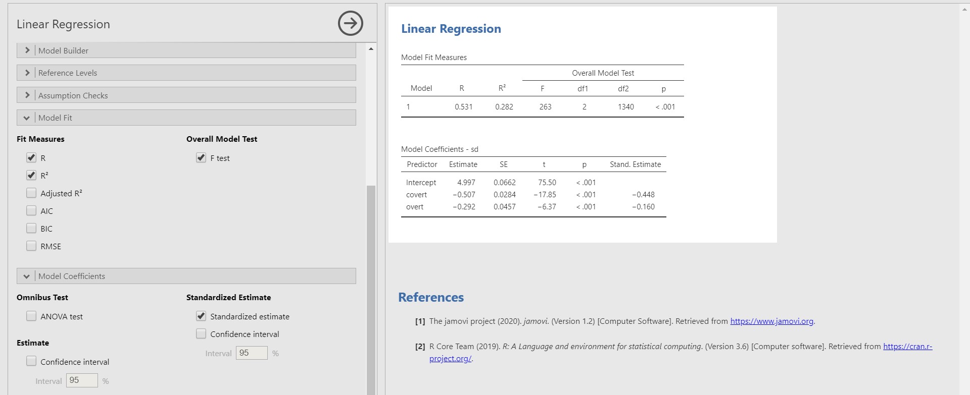
- The standardized regression coefficients can be found under the Stand. Estimate column in the Model Coefficients – sd table. The standardized regression coefficients are used to compare the effect sizes among predictors. These coefficients are scaled to one standard deviation.
- If one standard deviation of covert increases, 0.448 standard deviations of sd decreases.
- If one standard deviation of overt increases, 0.160 standard deviations of sd decreases.
- Therefore, the strength of covert in predicting sd is greater than that of overt.
- How about the F-test? Take a look at the row with number 1 in the table under Model Fit Measures. The F-statistic in the regression model indicates whether the model fits the data well. Let’s see the p-value of the F-statistic. Because the p-value of the F-statistic is lower than 0.001, the regression model fits significantly better than the model that does not contain any predictors.
3. t-test
- A t-test is an option when you are interested in examining whether the means of certain variables between the two groups significantly differ from each other.
- Go to the analyses ribbon -> Click T-Tests -> Click Independent Samples T-Test
- As an illustrative instance, let’s test whether the means of covert antisocial behavior (covert) between the respondents’ different ethnic backgrounds (Dutch) are significantly different.
- Move the covert variable under the Dependent Variables section and the Dutch variable under the Grouping Variable section.
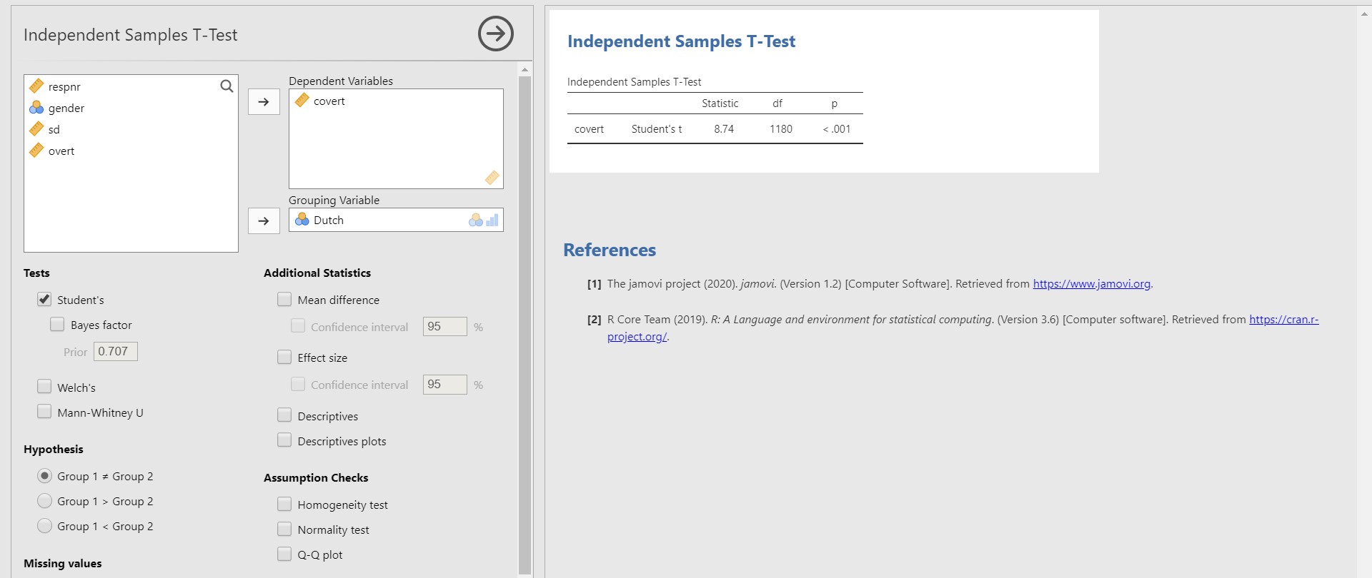
- Look at the table under Independent Samples T-Test. The p-value is lower than 0.001. Therefore, the two means of covert between two groups of the Dutch variable are significantly different from each other.
4. One-way analysis of variance
- If you are keen on investigating if the means are significantly different across groups, a one-way analysis of variance answers your question.
- Go to the analyses ribbon -> Click ANOVA -> Click One-Way ANOVA -> Move dependent variables of interest under the Dependent Variables section and one independent variable (also referred to as a factor) under the Grouping Variable section.
- Let’s investigate whether the means of the covert antisocial behavior (covert) are significantly different across respondents’ genders (gender).
- Before proceeding further, there is one thing we should do. According to the frequency table of gender in ‘III. Exploring data’, the gender variable has three categories: 0, 1, and 99. Since jamovi treats 99 as an independent category, which should not be the case, it is necessary to filter 99 out.
- Given that we have to manage data, can you guess where should we head for? Yes, data ribbon!
- Go to the data ribbon -> Click Filters button
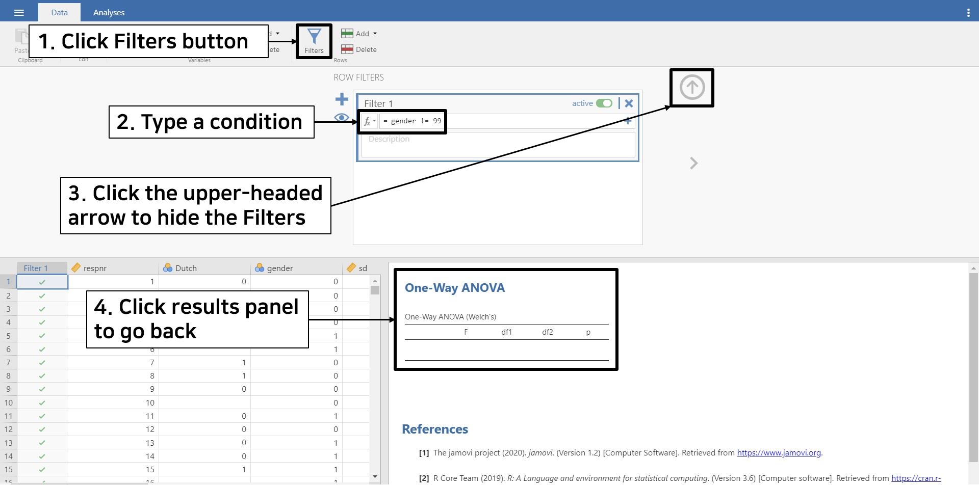
- Because we only need gender values other than 99, we will filter out 99 with the condition
gender != 99. Specifically, typegender(the variable name) and the symbol!=(not equal to), followed by typing99at the end. In doing so, we are telling jamovi that we will use gender values that are not equal to 99, hence using only 0 and 1 category. - Once you are done, jamovi automatically filters the value 99 in the gender variable out. Click the upper-headed arrow on the top right to hide the filter. Click the One-Way ANOVA section in the results panel to return to what we were working on.
- For readers who need a more detailed explanation about filters in jamovi, please visit here.
- Move covert under the Dependent Variables section and gender under the Grouping Variable section.
- Remember that at the beginning of ‘IV. Analysis and interpretation of data’, we assumed that all the assumptions are satisfied. This implies that the assumption of equal variances, one of the assumptions in performing ANOVA, is assumed to be met. However, the default setting of one-way ANOVA is that this assumption is not satisfied, so we uncheck Don’t assume equal (Welch’s) and check Assume equal (Fisher’s) under Variances in the options panel.
- If you want to test the assumption of homogeneous variances, check Homogeneity test under Assumption Checks in the options panel.
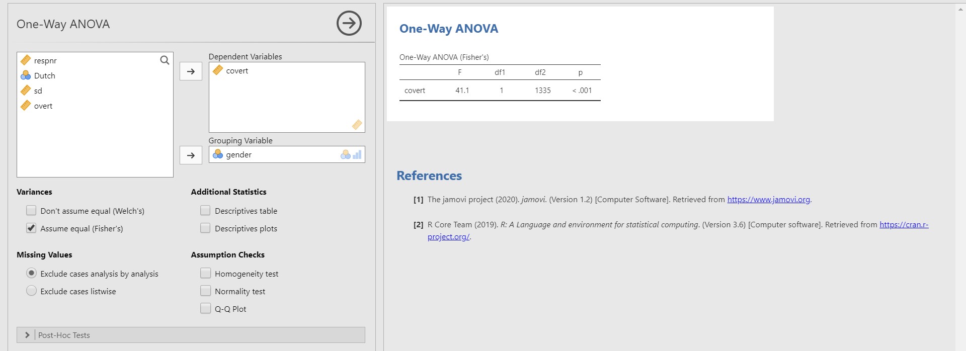
- Take a look at the table under One-Way ANOVA (Fisher’s). Since the p-value of covert is lower than 0.001, there are significant mean differences in covert between the two genders.
V. Feel the integrative vibe between jamovi and R
- One of the attractive points of jamovi aforementioned is the integration with R. This means that all the analyses we have conducted in jamovi can be transferrable to the R code. Furthermore, the R code can be used to implement analyses in jamovi. This is possible since jamovi is developed based on the R language. This section is devoted to feeling the integration between jamovi and R!
1. Syntax mode: Reproducibility of results
- Behind the conducted statistical analyses with simple mouse clicks, R code was programmed. Can’t you believe it? Then, let us show you by activating the syntax mode.
- As an example, let’s follow running the multiple regression analysis we did in ‘IV. Analysis and interpretation of data’. First, we do the steps with mouse clicks.
- Go to the analyses ribbon -> Click Regression -> Linear Regression -> Move sd to the Dependent Variables section and covert and overt to the Covariates section.
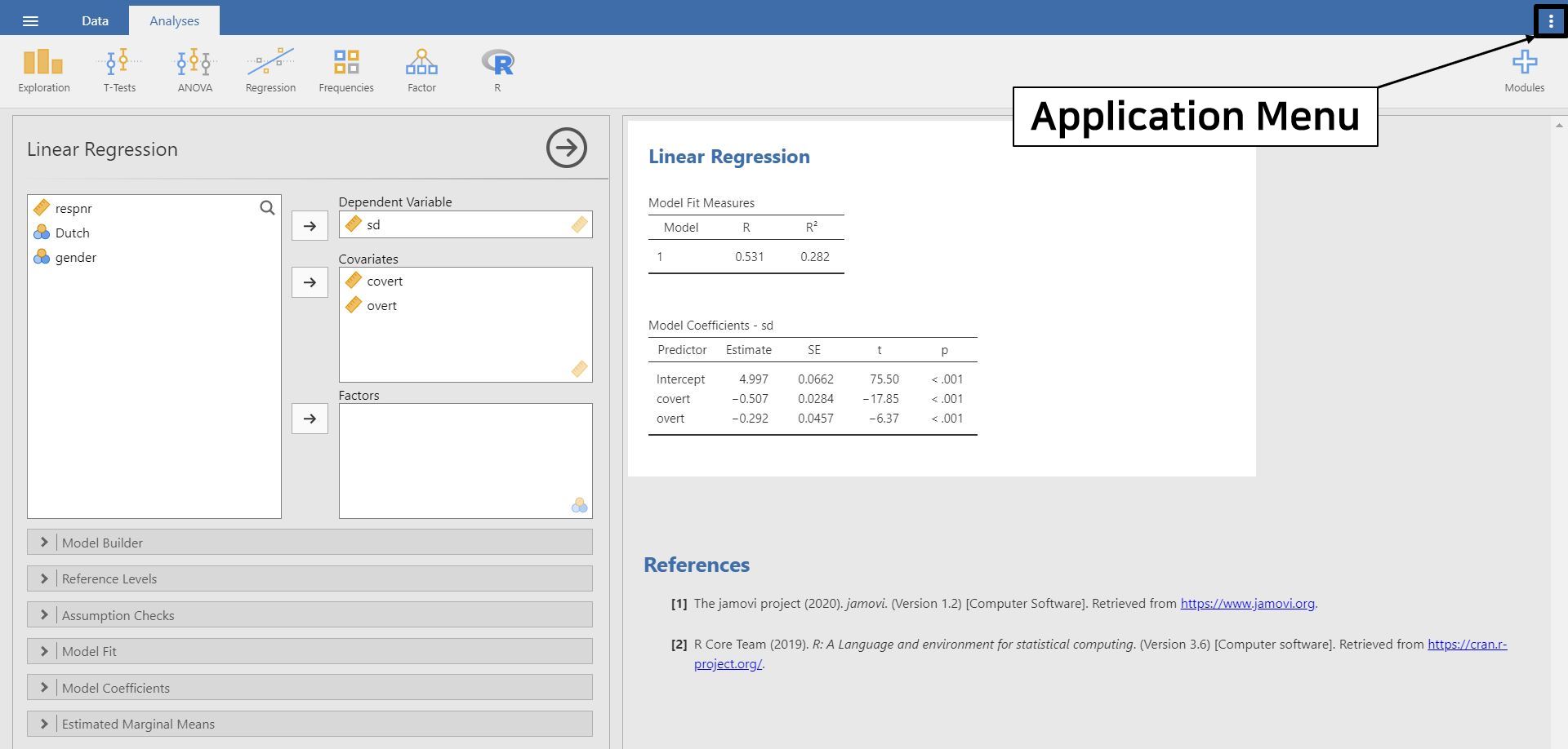
- At this point, focus your eyes on the three vertical dots at the top right of the jamovi screen (even farther than the plus button). This button is called the application menu, and we highlighted it with the black solid square! Click the application menu.
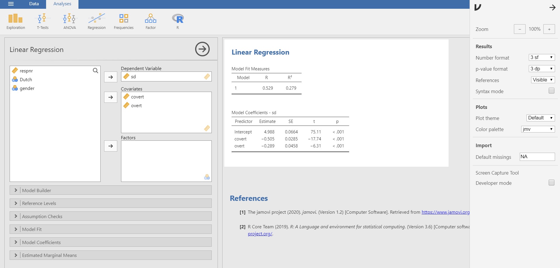
- Among the options in the pop-up, check Syntax mode. Be prepared to observe what happens on the results panel!
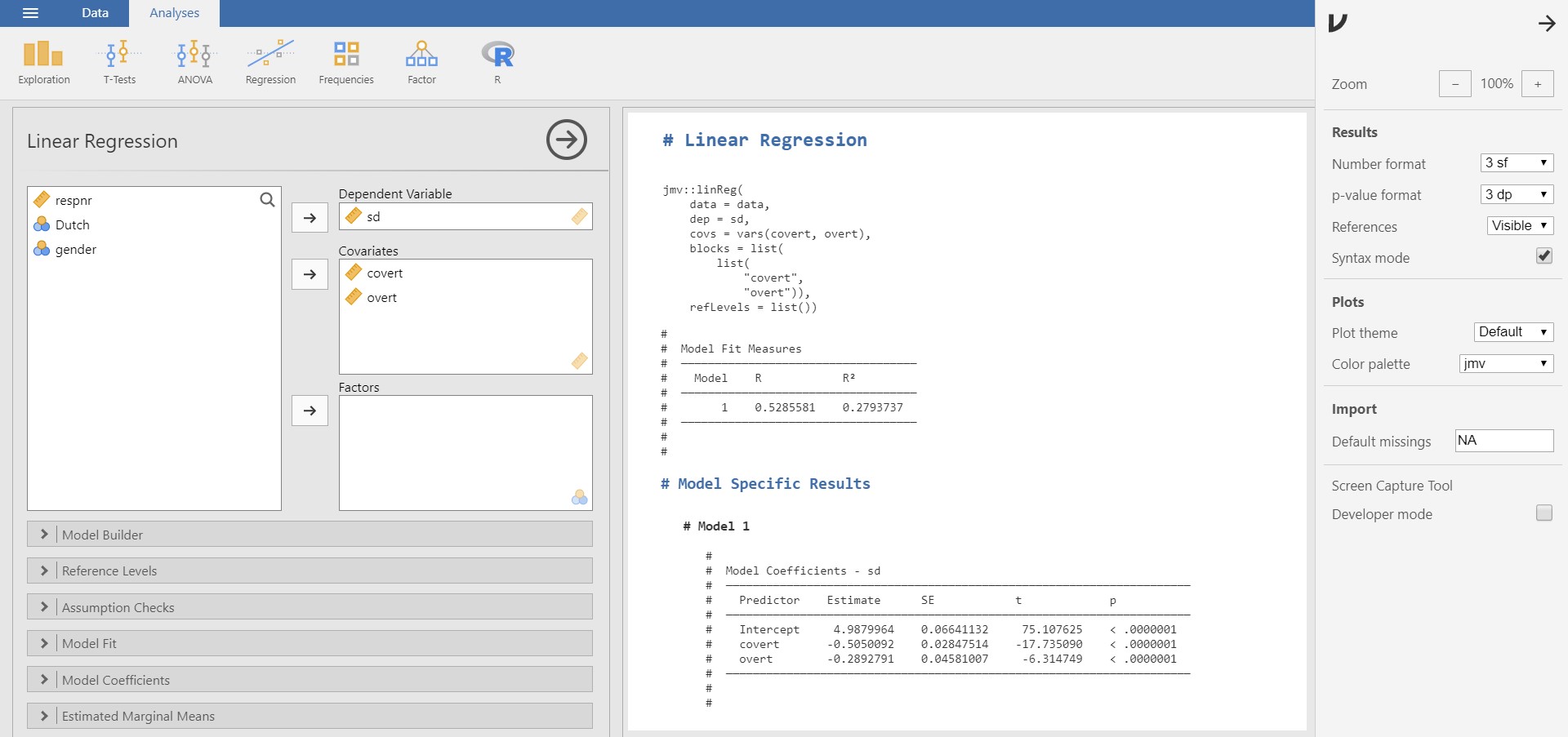
- Wow! What we have done with mouse clicks is represented as R code.
- You can always go back to the mode without the R code by unchecking Syntax mode.
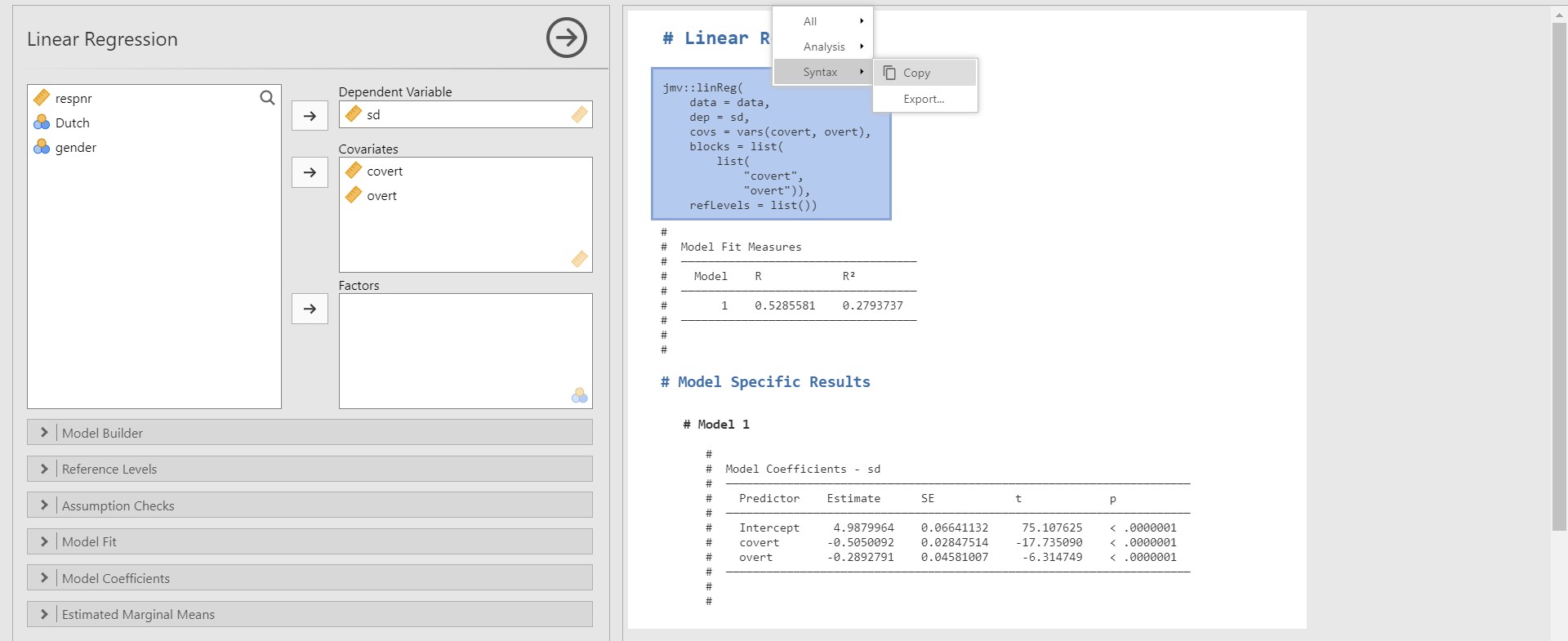
- If you right-click the corresponding R code and copy and paste it in R, you can reproduce the results.
- Please note that to run this copied code in R, (1) users should install the
jmvpackage in R, and (2) the dataset should be loaded with the object namedata. We provide the full code that works in R for interested readers. Be sure to specify the location of the file!
install.packages("jmv")
install.packages("haven")

library(jmv)
library(haven)

data <- read_sav("C:/Users/File Location/popular_regr_1.sav")

jmv::linReg(
    data = data,
    dep = sd,
    covs = vars(covert, overt),
    blocks = list(
        list(
            "covert",
            "overt")),
refLevels = list())- In this sense, jamovi enhances the reproducibility of results through the syntax mode.
2. Rj module: Inviting R to jamovi
- With the syntax mode, we uncovered the hidden R code behind the jamovi’s work. The Rj module, which is introduced here, is to conduct jamovi analyses with R programming.
- To do that, you should first install the Rj module. We are quite sure you are now familiar with installing modules following the steps in ‘I. Ice-breaking with jamovi’.
- Click the plus button -> jamovi library -> Find Rj module -> Click INSTALL
- If you click the analyses ribbon, you see that the new button with an R symbol was added.
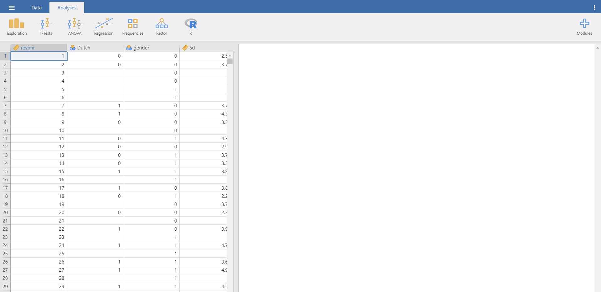
- Go to the analyses ribbon -> Click R -> Rj Editor
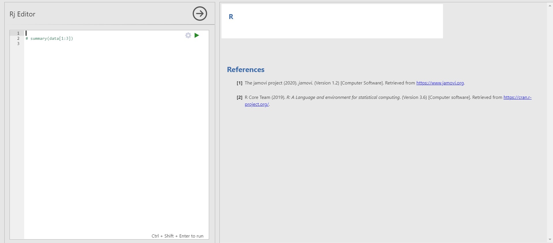
- In the options panel, there exists an editor. You can type the R code in the editor to run the analyses. Please note that our loaded data is referred to as ‘data’ in the Rj module.
- For example, to investigate the descriptive statistics of all the variables of our data, you can type the following code into the editor.
summary(data[1:6])- To implement the code, click the right-headed green triangle on the top right of the editor. You can also press Ctrl, Shift, and Enter together.
- Shortly, jamovi prints the descriptive statistics in the results panel.
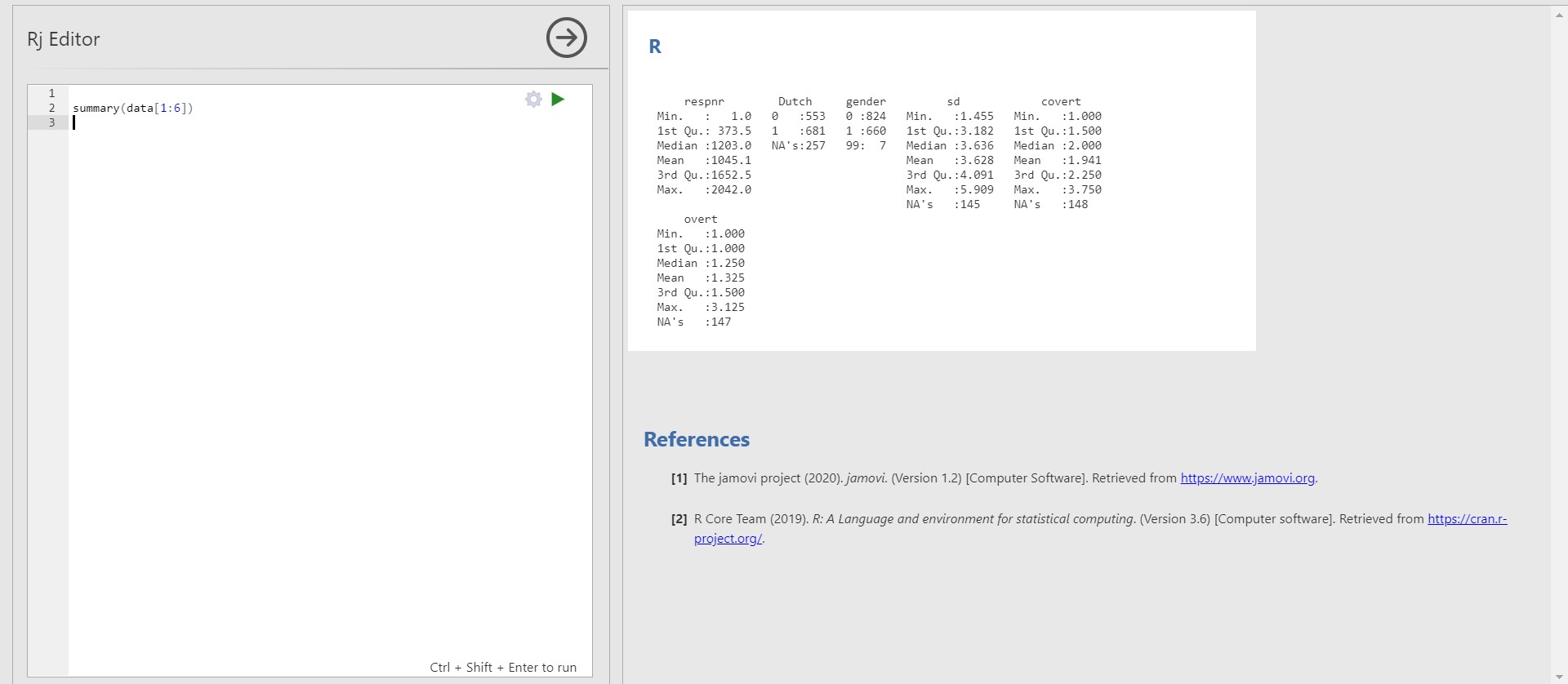
- In this way, you can anytime run the R code in jamovi. This functionality provides greater flexibility in running statistical analyses if you are an experienced R user.
- Since our focus of the current tutorial is not on R programming, we do not discuss further in the Rj module. Still, interested readers are encouraged to visit here to explore the Rj module.
- You may also find it useful to follow the tutorial R for beginners if you hope to learn the basics of R for statistical analyses!
3. Exporting results as R objects
- The power of integration between jamovi and R has not ended. Imagine we conducted a lot of analyses with jamovi and want to load them in R. Should we reiterate running the R code extracted from the syntax mode? Well, it might be a bit tedious.
- For us, jamovi provides the functionality where our analyses can be directly exported as R objects.
- Click file tab -> Export
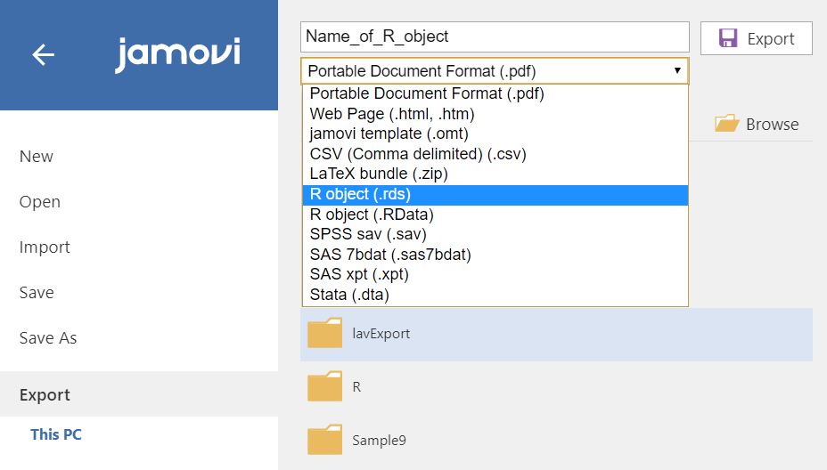
- After setting a name of an R object, choose either
.rdsor.RDataformat to export our works. What we need to do in R is to load the saved R objects. For the.rdsfile, usereadRDS()function. For the.RDatafile, useload()function. With this procedure, we can efficiently call our jamovi works in R!
VI. Epilogue
- Congratulations! You have reached the finish line of the introductory jamovi tutorial. We hope you enjoyed it.
- As mentioned at the beginning of ‘IV. Analysis and interpretation of data’, we only focused on statistical analyses from the frequentist statistics perspective. The focus for the ‘next step’ should be performing Bayesian statistical analyses with jamovi!
- Therefore, we strongly recommend you to follow our next tutorial jamovi for Bayesian analyses with default priors! It completely geared for Bayesian statistical analysis with easy steps. See you soon!
References
Anderson, E. (1936). The species problem in Iris. Annals of the Missouri Botanical Garden, 23(3), 457-509. https://doi.org/10.2307/2394164
Dolan, C. V., Oort, F. J., Stoel, R. D., & Wicherts, J. M. (2009). Testing measurement invariance in the target rotated multigroup exploratory factor model. Structural Equation Modeling: A Multidisciplinary Journal, 16(2), 295-314. https://doi.org/10.1080/10705510902751416
The jamovi project. (2020). jamovi (Version 1.2.27)[Computer software].
Van de Schoot, R. (2020). Popularity Dataset for Online Stats Training [Data set]. Zenodo. https://doi.org/10.5281/zenodo.3962123
Van de Schoot, R., & Depaoli, S. (2014). Bayesian analyses: Where to start and what to report. The European Health Psychologist, 16(2), 75-84.
Van de Schoot, R., Kaplan, D., Denissen, J., Asendorpf, J. B., Neyer, F. J., & Van Aken, M. A. (2014). A gentle introduction to Bayesian analysis: Applications to developmental research. Child development, 85(3), 842-860. https://doi.org/10.1111/cdev.12169
Van de Schoot, R., Van der Velden, F., Boom, J., & Brugman, D. (2010). Can at-risk young adolescents be popular and anti-social? Sociometric status groups, anti-social behaviour, gender and ethnic background. Journal of adolescence, 33(5), 583-592. https://doi.org/10.1016/j.adolescence.2009.12.004