Intro to Discrete-Time Survival Analysis in R
Qixiang Fang and Rens van de Schoot
Last modified: date: 14 October 2019
This tutorial provides the reader with a hands-on introduction to discrete-time survival analysis in R. Specifically, the tutorial first introduces the basic idea underlying discrete-time survival analysis and links it to the framework of generalised linear models (GLM). Then, the tutorial demonstrates how to conduct discrete-time survival analysis with the glm function in R, with both time-fixed and time-varying predictors. Some popular model evaluation methods are also presented. Lastly, the tutorial briefly extends discrete-time survival analysis with multilevel modelling (using the lme4 package) and Bayesian methods (with the brms package).
The tutorial follows this structure:
1. Preparation
2. Introduction to Discrete-Time Survival Analysis
3. Data “Scania”: Old Age Mortality in Scania, Southern Sweden
4. Data Preparation
5. Gompertz Regression
6. Model Evaluation: Goodness-of-Fit
7. Model Evaluation: Predictive Performance
8. Multilevel Discrete-Time Survival Analysis
9. Bayesian Discrete-Time Survival Analysis
Note that this tutorial is meant for beginners and therefore does not delve into very technical details or complex models. For a detailed introduction into GLM or multilevel models in R, see this tutorial. For an extensive overview of GLM models, see here. For more discrete-time survival analysis, check out Modeling Discrete Time-to-Event Data by Tutz & Schmid (2016). For more multilevel modelling, see Multilevel analysis: Techniques and applications.
1. Preparation
This tutorial expects:
– Installation of R package tidyverse for data manipulation and plotting with ggplot2;
– Installation of R package haven for reading sav format data;
– Installation of R packages lme4 for multilevel modelling (this tutorial uses version 1.1-18-1);
– Installation of R package jtools for handling of model summaries;
– Installation of R package ggstance for visualisation purposes;
– Installation of R package effects for plotting parameter effects;
– Installation of R package eha, which contains the data set we will use;
– Installation of R package discSurv, for discrete-time data manipulation and calculation of prediction error curves;
– Optional installation of R package brms for Bayesian discrete-time survival analysis (this tutorial uses version 2.9.0). Note that you do not need this package installed for the main codes of the tutorial to work. If interested, you can check out this tutorial for detailed installation instruction. Note that currently brms only works with R 3.5.3 or an earlier version;
– Basic knowledge of hypothesis testing and statistical inference;
– Basic knowledge of generalised linear models (GLM);
– Basic knowledge of coding in R;
– Basic knowledge of plotting and data manipulation with tidyverse.
2. Introduction to Discrete-Time Survival Analysis
If you are already familar with discrete-time survival analysis, you can proceed to the next section. Otherwise, click “Read More” to learn about it.
2.1. What Is Discrete-Time Survival Analysis?
Survival analysis is a body of methods commonly used to analyse time-to-event data, such as the time until someone dies from a disease, gets promoted at work, or has intercourse for the first time. The focus is on the modelling of event transition (i.e. from no to yes) and the time it takes for the event to occur. In comparison to other statistical methods, survival analysis has two particular advantages. First, it models the effects of both time-varying and time-fixed predictors on the outcome. For instance, whether a person develops the common cold may be influenced by both that person’s gender (which is in many cases a fixed variable that does not vary with time) and the weather conditions (which changes with time). Survival analysis can appropriately incorporate both time-fixed and time-varying factors into the same model, while most other modelling framework cannot. Second, survival analysis can take care of the right censoring issue in the data, with right censoring meaning that for some individuals the time when a transition (i.e. the target event) takes place is unknown, which poses missing data issues for other statistical approaches.
Many survival analysis techniques assume continuous measurement of time (e.g. Cox regression). However, in practice, data are often collected in discrete-time intervals, for instance, days, weeks and years, which violates the assumption of continous time in many standard survival analysis tools. Because of this reason, we need a special type of survival analysis for discrete-time data, namely discrete-time survival analysis. There are advantages to using discrete-time analysis, in comparison to its continuous-time counterpart. For example, discrete-time analysis has no problem with ties (i.e. multiple events occurring at the same time point) and it can be embedded into the generalised linear model (GLM) framework, as is shown next.
2.2. Hazard Function
The fundamental quantity used to assess the risk of event occurrence in a discrete-time period is hazard. Denoted by \(h_{is}\), discrete-time hazard is the conditional probability that individual \(i\) will experience the target event in time period \(s\), given that he or she did not experience it prior to time period \(s\). This translates into, for instance, the probability of person \(i\) dying during time \(s\) (e.g. day, month), given the individual did not die earlier. The hazard function can be formalised as follows:
\[h_{is} = P(T_{i} = s\;|\;T_{i} \geq s)\]
where \(T\) represent a discrete random variable whose values \(T_i\) indicate the time period \(s\) when individual \(i\) experiences the target event. The hazard function, thus, represents the probability that the event will occur in the current time period \(s\), given that it must occur now, or sometime later.
The value of discrete-time hazard in time period \(s\) can be estimated as:
\[\tilde{h}_s = \frac{\text{number of events}_{s}}{\text{number at risk}_{s}}\]
where “\(\text{number events}_{s}\)” represents the number of individuals who experience the target event in time \(s\), while “\(\text{number at risk}_{s}\)” indicates the number of people at risk of the event during time \(s\).
2.3. Discrete-Time Regression Models
A general representation of the hazard function that connects the hazard \(h_{is}\) to a linear predictor \(\eta\) is
\[\eta = g(h_{is}) = \gamma_{0s} + x_{is}\gamma\]
where \(g(.)\) is a link function. It links the hazard and the linear predictor \(\eta = \gamma_{0s} + x_{is}\gamma\), which contains the effects of covariates for individual \(i\) in time period \(s\). The intercept \(\gamma_{0s}\) is assumed to vary over time, whereas the parameter \(\gamma\) is fixed. Since hazards are probabilities restricted to the interval [0, 1], natural candidates for the response function \(g(.)\) are, for instance, the logit link and the Gompertz link (also called complementary log-log link). Both of them are frequent choices in discrete-time survival analysis. The corresponding hazard functions become
\[
logit: h_{is} = \exp(\eta)/(1+\exp(\eta)) \\
Gompertz: h_{is} = 1 – \exp(-\exp(\eta))
\]
Both link functions are appropriate in most cases. In fact, when the underlying hazards are small, both link functions usually lead to very similar parameter estimates. However, there are two differences. First, the two links result in different interpretations of the estimated parameters. In a logistic model (i.e. using the logit link), the exponential term of a parameter estimate quantifies the difference in the value of the odds per unit difference in the predictor, while in the Gompertz model it is the value of the hazard (i.e. which is a probability). Therefore, the Gompertz link results in a more intuitive model interpretation. Second, the Gompertz link assumes the underlying distribution of time to be continuous, but for practical reasons the measurement is discrete. Where it is safe to assume a continuous underlying distribution of time, we recommend using the Gompertz link and thus one would also benefit from more interpretable model estimates; otherwise, the logit link.
2.4. The GLM Framework and Person-Period Data
The total negative log-likelihood of the discrete survival regression model, assuming random (right) censoring, is given by
\[
-l \propto \sum_{i=1}^n\sum_{s=1}^{t_{i}} y_{is}\log h_{is} + (1-y_{is})log(1- h_{is})
\]
where \(y_{is} = 1\) if the target event occurs for individual \(i\) during time period \(s\), and \(y_{is} = 0\) otherwise; \(n\) refers to the total number of individuals; \(t_i\) the observed censored time for individual \(i\). This negative log-likelihood is equivalent to that of a binary response model (e.g. binary logistic regression). This analogue allows us to use software designed for binary response models for model estimation, with only two modifications. First, the distribution function is Gompertz (if not logit). Second, the number of binary observations in the discrete survival model depends on the observed censoring and lifetimes. Thus, the number of binary observations is \(\sum_{i = 1}^{n}\sum_{s = 1}^{t_{i}}\). This requires the so-called Person-Period data format, where there is a separate row for each individual \(i\) for each period \(s\) when the person is observed. In each row a variable indicates whether an event occurs. The event occurs in the last observed period unless the observation has been censored.
Below is an exemplar Person-Period data set, containing observations from three persons.
##    id time event gender employed
## 1   1    1     0   male      yes
## 2   1    2     0   male      yes
## 3   1    3     1   male       no
## 4   2    1     1 female       no
## 5   3    1     0 female      yes
## 6   3    2     0 female      yes
## 7   3    3     0 female       no
## 8   3    4     0 female      yes
## 9   3    5     0 female      yes
## 10  3    6     0 female      yes
As we can see in this example, a person (indicated by column id) has multiple rows for all the time points when the person is observed. A person is censored when he/she has experienced the target event (i.e. id = 1 and id = 2), or when the data collection ends systematically at time point 6 (i.e. id = 3). Both time-fixed variables (e.g. gender) and time-varying variables (e.g. employment status) can be easily integrated into such a data format.
One may wonder whether the analysis of the multiple records in a Person-Period data set yields appropriate parameter estimates, standard errors and goodness-of-fit statistics when the multiple records for each person in the data set do not appear to be independent from each other. This is not an issue in discrete time survival analysis because the hazard function describes the conditional probability of event occurrence, where the conditioning depends on the individual surviving until each specific time period \(s\) and his or her values for the substantive predictors in each time period. Therefore, records in the person-period data need to only assume conditional independence.
The next section details the exampler data (Scania Data) in this tutorial, followed by a demonstration of Gompertz regression and a brief introduction to its multilevel and Bayesian extension.
3. Data “Scania”: Old Age Mortality in Scania, Southern Sweden
The data used in this tutorial is Scania, offered by The Scanian Economic Demographic Database (Lund University, Sweden). The data consists of old-age life histories from 1 January 1813 to 31 December 1894 in Scania, Southern Sweden. Only life histories above age 50 are included. The data set has 9 variables (not all will be considered in this study). They are:
id: identification number of the person;
enter: start age of the person (beginning time interval);
exit: stop age of the person (cencored/final time interval);
event: indicator of death at a corresponding time interval;
birthdate: birthdate of the person;
sex: gender, a factor with levels “male” and “female”;
parish: one of five parishes in Scania, factor variable;
ses: socio-economic status at age 50, a factor with levels “upper” and “lower”;
immigrant: a factor with levels “no” and “yes”.
This data set comes with the R package eha. Note that in this data set, there is no time-varying predictor. Therefore, we will manually add a time-varying variable “foodprices” from the logrye data set that is also available in the eha package. “logrye” consists of yearly rye prices from 1801 to 1894 in Scania. Rye prices are used as an indicator for food prices.
The main research question that this tutorial seeks to answer using the “Scania” data is: What are the effects of gender, socio-economic status, immigrant status, and food prices on a person’s conditional probability of dying during a given time interval?
4. Data Preparation
4.1. Load necessary packages
# if you dont have these packages installed yet, please use the install.packages("package_name") command.
library(lme4) # for multilevel models
library(tidyverse) # for data manipulation and plots
library(effects) #for plotting parameter effects
library(jtools) #for transformaing model summaries
library(eha) #for the data sets used in this tutorial
library(discSurv) #discrete-time survival analysis tool kit
#library(brms) #Bayesian discrete-time survival analysis
4.2. Import Data
data("scania")
head(scania)
## id enter exit event birthdate sex parish ses immigrant
## 29 1 50 59.242 1 1781.454 male 1 lower no
## 66 2 50 53.539 0 1821.350 male 1 lower yes
## 70 3 50 62.155 1 1788.936 male 1 lower yes
## 83 4 50 65.142 1 1796.219 female 1 lower yes
## 100 5 50 51.280 0 1822.713 male 1 lower yes
## 132 6 50 70.776 1 1813.547 female 1 lower yesNote that the data set follows a Person-Level format, where each person has only one row of data containing summary information about the duraction of observation. We will convert it to Person-Period format later that is suitable for discrete-time survival analysis.
4.3. Convert to Discrete-Time Measurement
The original data is measured on continuous time scale. To render the data suitable for discrete-time analysis, we convert the time variables (enter, exit and birthdate) to discrete-time measurements.
Scania_Person <- scania %>%
  mutate(exit = ceiling(exit),
         birthdate = floor(birthdate),
         spell = exit - enter) %>% #spell refers to the observed duration of a person
  mutate(enter = enter - 50,
         exit = exit - 50)

head(Scania_Person)
## id enter exit event birthdate sex parish ses immigrant spell
## 1 1 0 10 1 1781 male 1 lower no 10
## 2 2 0 4 0 1821 male 1 lower yes 4
## 3 3 0 13 1 1788 male 1 lower yes 13
## 4 4 0 16 1 1796 female 1 lower yes 16
## 5 5 0 2 0 1822 male 1 lower yes 2
## 6 6 0 21 1 1813 female 1 lower yes 214.4. Divide Data into Training (80%) and Test (20%) Sets
Normally, we are not only interested in explaining a data set, but also curious about the generalisibility of the results to unseen cases. That is to say, we want to know if our model, trained on some data, performs well on some other data, which can be evaluated using some criteria (e.g. mean squared error; correct classification rate). For this reason, we divide our current data randomly into two parts: a training data set comprising 80% of the cases with which we build a discrete-time survival model; a test data set comprising 20% of the cases which we use to evaluate the model that we train on the training data set.
set.seed(123)
Scania_Person_Train <- sample_frac(Scania_Person, 0.8)
Scania_Person_Test <- Scania_Person[!Scania_Person$id %in% Scania_Person_Train$id,]
4.6. Person-Period Format
Now we convert both the training and the test data into Person-Period format, using the dataLong function from the discSurv package. Then, we use the left_join function from tidyverse to join the scania data with the logrye data (also supplied by the eha package) for a time-dependent variable about food prices of a given year.
#convert the training set
Scania_PersonPeriod_Train <- dataLong(dataSet = Scania_Person_Train,
                                      timeColumn = "spell",
                                      censColumn = "event",
                                      timeAsFactor = F) %>%
  as_tibble() %>%
  mutate(enter = timeInt - 1,
         age = enter + 50) %>%
  select(-obj, -event, -exit) %>%
  rename(event = y,
         exit = timeInt) %>%
  mutate(year = age + birthdate) %>%
  select(id, enter, exit, event, everything()) %>%
  left_join(logrye, by = "year") #joined with the `logrye` data for a variable on yearly food prices

head(Scania_PersonPeriod_Train)
## # A tibble: 6 x 13
## id enter exit event birthdate sex parish ses immigrant spell
## <int> <dbl> <int> <dbl> <dbl> <fct> <fct> <fct> <fct> <dbl>
## 1 556 0 1 0 1778 fema~ 4 lower yes 9
## 2 556 1 2 0 1778 fema~ 4 lower yes 9
## 3 556 2 3 0 1778 fema~ 4 lower yes 9
## 4 556 3 4 0 1778 fema~ 4 lower yes 9
## 5 556 4 5 0 1778 fema~ 4 lower yes 9
## 6 556 5 6 0 1778 fema~ 4 lower yes 9
## # ... with 3 more variables: age <dbl>, year <dbl>, foodprices <dbl>#convert the test set
Scania_PersonPeriod_Test <- dataLong(dataSet = Scania_Person_Test,
timeColumn = "spell",
censColumn = "event",
timeAsFactor = F) %>%
as_tibble() %>%
mutate(enter = timeInt - 1,
age = enter + 50) %>%
select(-obj, -event, -exit) %>%
rename(event = y,
exit = timeInt) %>%
mutate(year = age + birthdate) %>%
select(id, enter, exit, event, everything()) %>%
left_join(logrye, by = "year")
head(Scania_PersonPeriod_Test)## # A tibble: 6 x 13
## id enter exit event birthdate sex parish ses immigrant spell
## <int> <dbl> <int> <dbl> <dbl> <fct> <fct> <fct> <fct> <dbl>
## 1 27 0 1 0 1819 fema~ 1 upper yes 2
## 2 27 1 2 0 1819 fema~ 1 upper yes 2
## 3 32 0 1 0 1814 fema~ 1 lower yes 19
## 4 32 1 2 0 1814 fema~ 1 lower yes 19
## 5 32 2 3 0 1814 fema~ 1 lower yes 19
## 6 32 3 4 0 1814 fema~ 1 lower yes 19
## # ... with 3 more variables: age <dbl>, year <dbl>, foodprices <dbl>5. Gompertz Regression
5.1. Fit a Baseline Gompertz Regression Model
An important consideration in discrete-time survival analysis concerns the specification of the intercept \(\gamma_{0s}\) in model equation \(\eta = g(h_{is}) = \gamma_{0s} + x_{is}\gamma\). The intercept term \(\gamma_{0s}\) can be interpreted as a baseline hazard, which is present for any given set of covariates. The specification of the intercept \(\gamma_{0s}\) is very flexible, varying from giving all discrete time points their own parameters to specifying a single linear term. To determine the specification of \(\gamma_{0s}\), we can visually inspect the relationship between the time points (exit) and the cloglog transformation of the observed hazards. See below.
Scania_PersonPeriod_Train %>%
  group_by(exit) %>%
  summarise(event = sum(event),
            total = n()) %>%
  mutate(hazard = event/total) %>%
  ggplot(aes(x = exit, y = log(-log(1-hazard)))) +
  geom_point() +
  geom_smooth()
## `geom_smooth()` using method = 'loess' and formula 'y ~ x'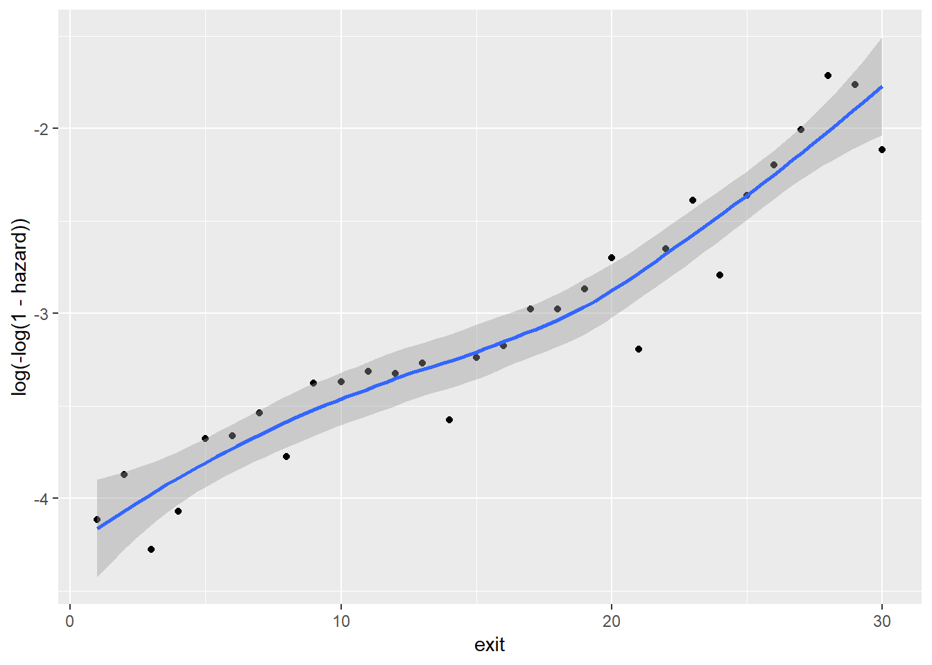
We can see that the relationship between time (exit) and the cloglog(hazard) is almost a linear straight line. Therefore, we set up the baseline model by specifying a single linear term for \(\gamma_{0s}\). See below.
Note that the specification of a Gompertz model is similar to a binary logistic regression model (using the glm function). The only difference is that we need to set the link function as “cloglog”.
Gompertz_Model_Baseline <- glm(formula = event ~ exit,
                               family = binomial(link = "cloglog"),
                               data = Scania_PersonPeriod_Train)

summary(Gompertz_Model_Baseline)
##
## Call:
## glm(formula = event ~ exit, family = binomial(link = "cloglog"),
## data = Scania_PersonPeriod_Train)
##
## Deviance Residuals:
## Min 1Q Median 3Q Max
## -0.5262 -0.3105 -0.2386 -0.1976 2.8879
##
## Coefficients:
## Estimate Std. Error z value Pr(>|z|)
## (Intercept) -4.237533 0.073795 -57.42 <2e-16 ***
## exit 0.075346 0.004202 17.93 <2e-16 ***
## ---
## Signif. codes: 0 '***' 0.001 '**' 0.01 '*' 0.05 '.' 0.1 ' ' 1
##
## (Dispersion parameter for binomial family taken to be 1)
##
## Null deviance: 7211.1 on 22334 degrees of freedom
## Residual deviance: 6897.5 on 22333 degrees of freedom
## AIC: 6901.5
##
## Number of Fisher Scoring iterations: 6From the model summary above, we can see a significant and positive relationship between exit and hazard. This baseline effect of time (i.e. exit) on hazards is the same for all individuals and changes only with regards to time (i.e. exit). For instance, at time point 30 (exit = 30) (which means that the person’s age is about 50 + 30 = 80), the baseline hazard for all individuals is: 1-exp(-exp(-4.237533+0.075346*30)) = 0.13. This means that at age 80, the conditional probability (hazard) of dying for an individual in that year (without factoring in any other information) is 0.13.
To ease the interpretaion, we can exponentiate the model estimates, using the summ function from the jtools package.
summ(Gompertz_Model_Baseline, exp = T) #exp = T means that we want exponentiated estimates## MODEL INFO:
## Observations: 22335
## Dependent Variable: event
## Type: Generalized linear model
## Family: binomial
## Link function: cloglog
##
## MODEL FIT:
## <U+03C7>²(1) = 313.55, p = 0.00
## Pseudo-R² (Cragg-Uhler) = 0.05
## Pseudo-R² (McFadden) = 0.04
## AIC = 6901.51, BIC = 6917.53
##
## Standard errors: MLE
##
## | | exp(Est.)| 2.5%| 97.5%| z val.| p|
## |:-----------|---------:|----:|-----:|------:|----:|
## |(Intercept) | 0.01| 0.01| 0.02| -57.42| 0.00|
## |exit | 1.08| 1.07| 1.09| 17.93| 0.00|An estimate of 1.08 means that, for one unit increase in exit (i.e. one additional observed year for a person), the probability (i.e. hazard) of the person dying, given that he/she survived the last time period, increases by 1.08 – 1 = 8%.
5.2. Fit a Full Gompertz Regression Model
To answer the research question (i.e. What are the effects of gender, socio-economic status, immigrant status, and food prices on a person’s conditional probability of dying during a given time interval?), we would want to fit a Gompertz regression model that includes all the variables of interest (i.e. sex, ses, immigrant and foodprices). Before we specify the model, it might be interesting to also visually examine the relationship between these variables and cloglog(hazard).
Between sex and cloglog(hazard):
Scania_PersonPeriod_Train %>%
  group_by(exit, sex) %>%
  summarise(event = sum(event),
         total = n()) %>%
  mutate(hazard = event/total) %>%
  ggplot(aes(x = exit,
             y = log(-log(1-hazard)),
             col = sex)) +
  geom_point() +
  geom_smooth()
## `geom_smooth()` using method = 'loess' and formula 'y ~ x'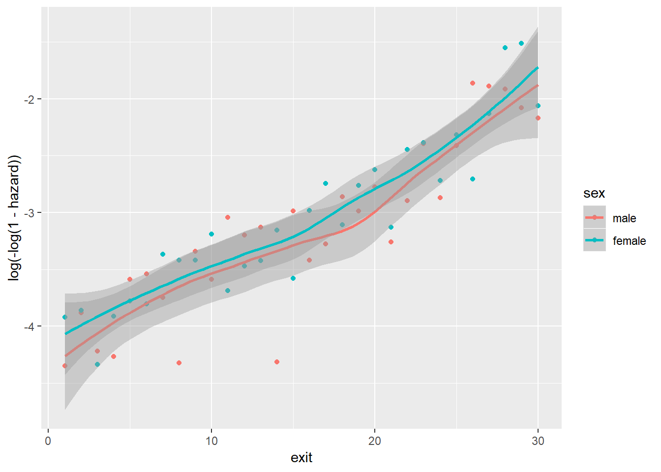
Between ses and cloglog(hazard):
Scania_PersonPeriod_Train %>%
  group_by(exit, ses) %>%
  summarise(event = sum(event),
         total = n()) %>%
  mutate(hazard = event/total) %>%
  ggplot(aes(x = exit,
             y = log(-log(1-hazard)),
             col = ses)) +
  geom_point() +
  geom_smooth()
## `geom_smooth()` using method = 'loess' and formula 'y ~ x'
Between immigrant and cloglog(hazard):
Scania_PersonPeriod_Train %>%
  group_by(exit, immigrant) %>%
  summarise(event = sum(event),
         total = n()) %>%
  mutate(hazard = event/total) %>%
  ggplot(aes(x = exit,
             y = log(-log(1-hazard)),
             col = immigrant)) +
  geom_point() +
  geom_smooth()
## `geom_smooth()` using method = 'loess' and formula 'y ~ x'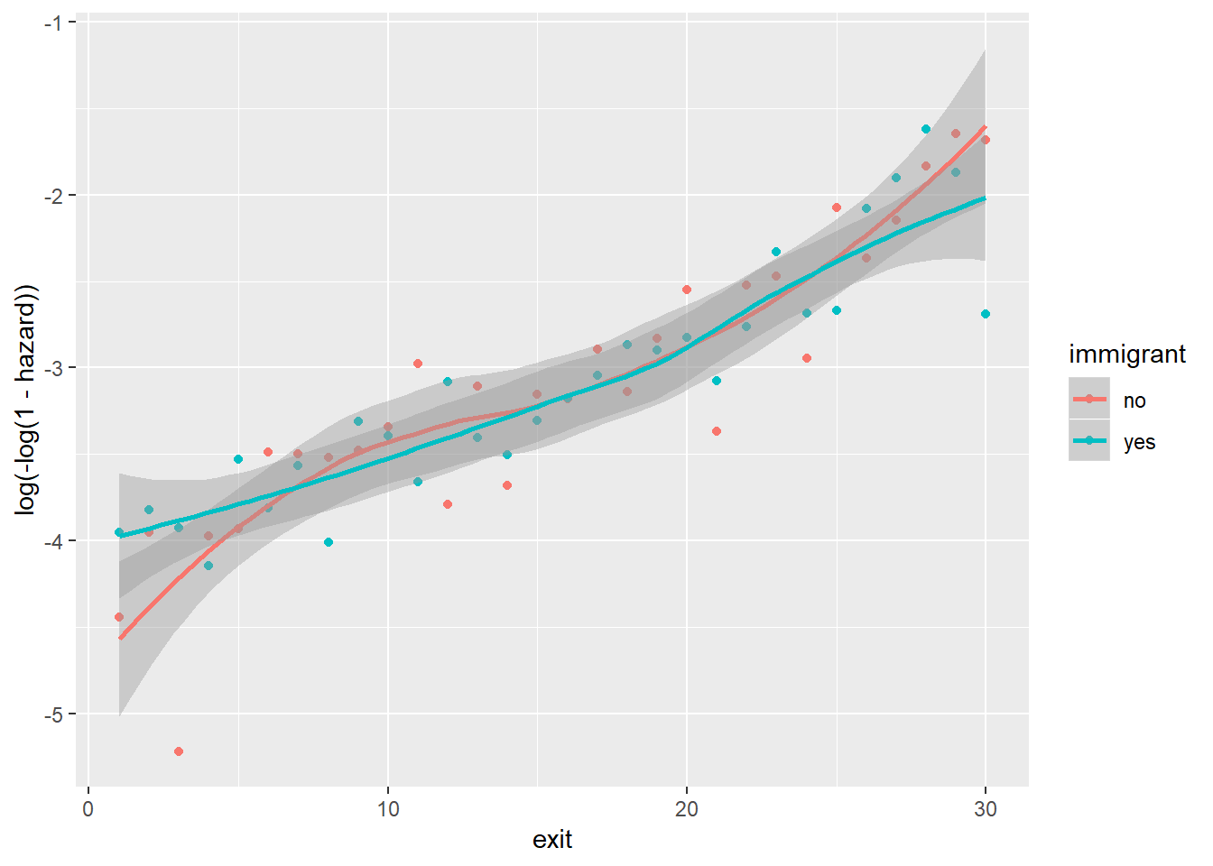
Between foodprices and cloglog(hazard):
Scania_PersonPeriod_Train %>%
  mutate(foodprices = cut_interval(foodprices, 10, labels = F)) %>%
  group_by(foodprices) %>%
  summarise(event = sum(event),
            total = n()) %>%
  mutate(hazard = event/total) %>%
  ggplot(aes(x = foodprices, y = log(-log(1-hazard)))) +
  geom_point() +
  geom_smooth(method = "lm")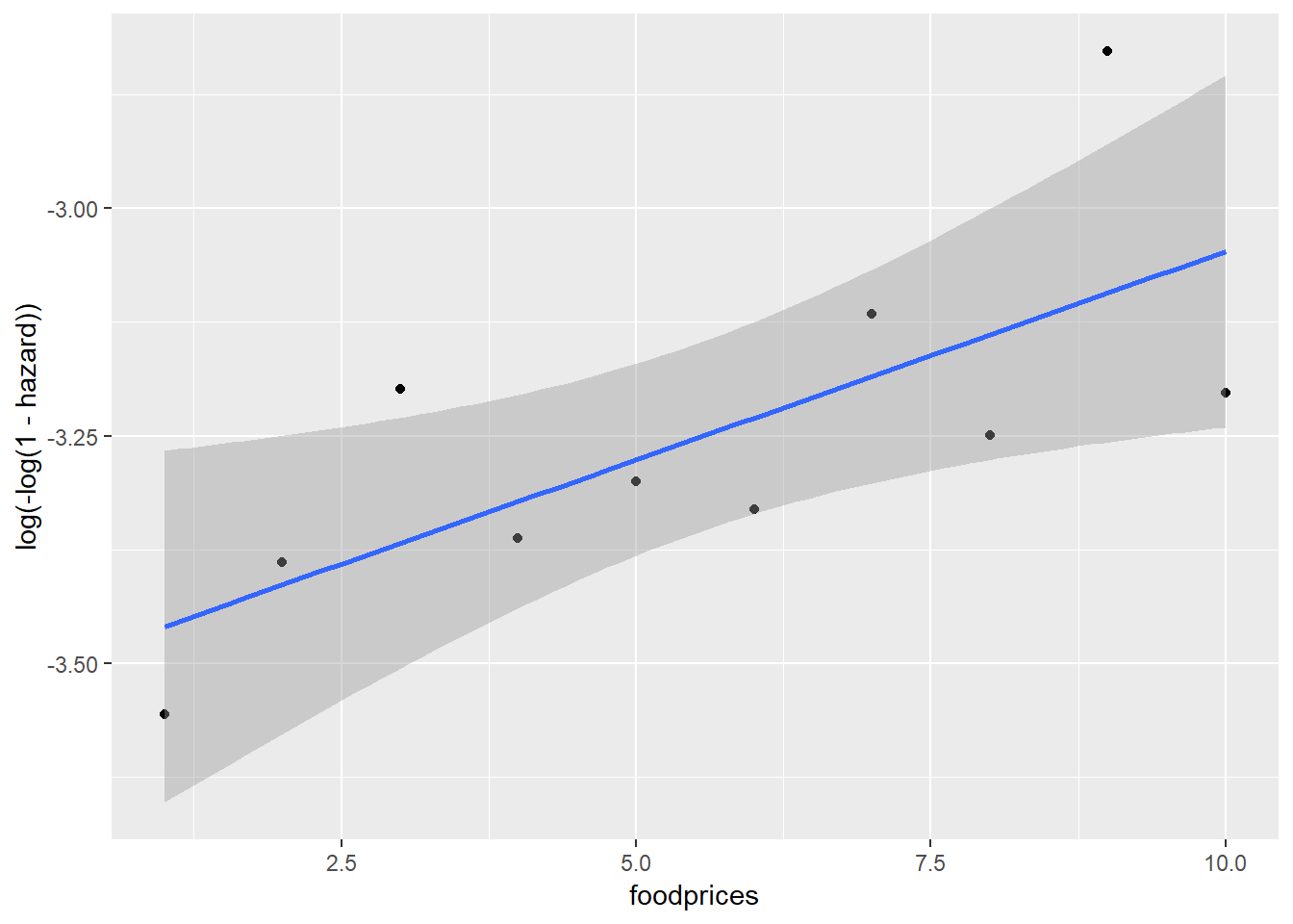
Note that because foodprices is a continous variable, we cut it into 10 intervals of equal lengths (indicated by 1 through 10). As we can see, at almost any given point in time (exit), different groups of the sex, ses and immigrant variables, respectively, have similar cloglog(hazard) values, indicated by the largely overlapped uncertainty regions. Therefore, it is unlikely that these three variables contribute to the prediction of hazards on top of the baseline intercept term (exit). On the other hand, foodprices seems to be positively and linearly related to cloglog(hazard).
Now we fit the full model with all the variables just examined.
Gompertz_Model_Full <- glm(formula = event ~ exit + sex + ses + immigrant + foodprices,
                           family = binomial(link = "cloglog"),
                           data = Scania_PersonPeriod_Train)

summary(Gompertz_Model_Full)
##
## Call:
## glm(formula = event ~ exit + sex + ses + immigrant + foodprices,
## family = binomial(link = "cloglog"), data = Scania_PersonPeriod_Train)
##
## Deviance Residuals:
## Min 1Q Median 3Q Max
## -0.5822 -0.3055 -0.2356 -0.1961 2.9381
##
## Coefficients:
## Estimate Std. Error z value Pr(>|z|)
## (Intercept) -4.306098 0.112021 -38.440 < 2e-16 ***
## exit 0.075387 0.004205 17.929 < 2e-16 ***
## sexfemale 0.077144 0.069053 1.117 0.26392
## seslower 0.036178 0.086316 0.419 0.67512
## immigrantyes -0.009161 0.069502 -0.132 0.89514
## foodprices 0.549623 0.206521 2.661 0.00778 **
## ---
## Signif. codes: 0 '***' 0.001 '**' 0.01 '*' 0.05 '.' 0.1 ' ' 1
##
## (Dispersion parameter for binomial family taken to be 1)
##
## Null deviance: 7211.1 on 22334 degrees of freedom
## Residual deviance: 6888.9 on 22329 degrees of freedom
## AIC: 6900.9
##
## Number of Fisher Scoring iterations: 6Confirming our previous visual observations, ses, ses, and immigrant do not significantly predict the outcome, while exit and foodprices are significantly and positively related to hazards. To ease the interpretation, we exponentiate the estimates:
summ(Gompertz_Model_Full, exp = T)## MODEL INFO:
## Observations: 22335
## Dependent Variable: event
## Type: Generalized linear model
## Family: binomial
## Link function: cloglog
##
## MODEL FIT:
## <U+03C7>²(5) = 322.18, p = 0.00
## Pseudo-R² (Cragg-Uhler) = 0.05
## Pseudo-R² (McFadden) = 0.04
## AIC = 6900.88, BIC = 6948.96
##
## Standard errors: MLE
##
## | | exp(Est.)| 2.5%| 97.5%| z val.| p|
## |:------------|---------:|----:|-----:|------:|----:|
## |(Intercept) | 0.01| 0.01| 0.02| -38.44| 0.00|
## |exit | 1.08| 1.07| 1.09| 17.93| 0.00|
## |sexfemale | 1.08| 0.94| 1.24| 1.12| 0.26|
## |seslower | 1.04| 0.88| 1.23| 0.42| 0.68|
## |immigrantyes | 0.99| 0.86| 1.14| -0.13| 0.90|
## |foodprices | 1.73| 1.16| 2.60| 2.66| 0.01|foodprices seems to have a very strong effect on the outcome hazards. For one unite increase in food prices, a person’s probabilty (hazard) of dying is increased by 73%, at any given time point. However, note that the range of foodprices is only between -0.40 and 0.40; it is, therefore, impossible that foodprices increases by 1. Because of this, it makes more sense to interpret the standardised estimates by setting scale = T:
summ(Gompertz_Model_Full, exp = T, scale = T)## MODEL INFO:
## Observations: 22335
## Dependent Variable: event
## Type: Generalized linear model
## Family: binomial
## Link function: cloglog
##
## MODEL FIT:
## <U+03C7>²(5) = 322.18, p = 0.00
## Pseudo-R² (Cragg-Uhler) = 0.05
## Pseudo-R² (McFadden) = 0.04
## AIC = 6900.88, BIC = 6948.96
##
## Standard errors: MLE
##
## | | exp(Est.)| 2.5%| 97.5%| z val.| p|
## |:-----------|---------:|----:|-----:|------:|----:|
## |(Intercept) | 0.03| 0.03| 0.04| -37.93| 0.00|
## |exit | 1.77| 1.66| 1.88| 17.93| 0.00|
## |sex | 1.08| 0.94| 1.24| 1.12| 0.26|
## |ses | 1.04| 0.88| 1.23| 0.42| 0.68|
## |immigrant | 0.99| 0.86| 1.14| -0.13| 0.90|
## |foodprices | 1.10| 1.02| 1.18| 2.66| 0.01|
##
## Continuous predictors are mean-centered and scaled by 1 s.d.Now, we know that hazards increase by 10% with a standard deviation increase in foodprices, assuming everything else stays constant.
5.3. Visualisation of Parameter Effects
To make the interpretation of the parameter effects even easier, we can use the plot_summs function from the joots package. It is useful to set exp = T and scale = T, so that we can exponentiated standardised estimates that are easier to interprete than the raw numbers.
plot_summs(Gompertz_Model_Full, exp = T, scale = T)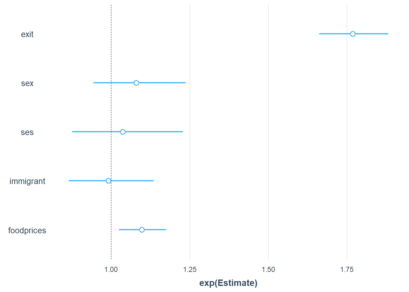
Now we can see that the strongest predictor of the outcome is exit, followed by foodprices. In contrast, sex, ses, and immigrant are unlikely important predictors because their uncertainty intervals overlap with 1, which indicates likely no effect.
Alternatively, we can use the allEffects function from the effects package to visualise the parameter effects. See below.
plot(allEffects(Gompertz_Model_Full))
Note that in these plots, the y scales refer to the predicted hazards (conditional probability of death). Such plots are helpful when the model uses a link (e.g. logit) that results in less interpretable model estimates, because probabilities (hazards) are more interpretable than, for example, odds. The probability scores for each variable are calculated by assuming that the other variables in the model are constant and take on their average values. Note that the confidence intervals for the estimates are also included to give us some idea of the uncertainties.
Note that the notion of average ses, sex and immigrant may sound strange, given they are categorical variables (i.e. factors). If you are not comfortable with the idea of assuming an average factor, you can specify your intended factor level as the reference point, by using the fixed.predictors = list(given.values = ...) argument in the allEffects function. See below:
plot(allEffects(Gompertz_Model_Full,
                fixed.predictors = list(given.values=c(sexfemale=0,
                                                       seslower = 0,
                                                       immigrantyes = 0))))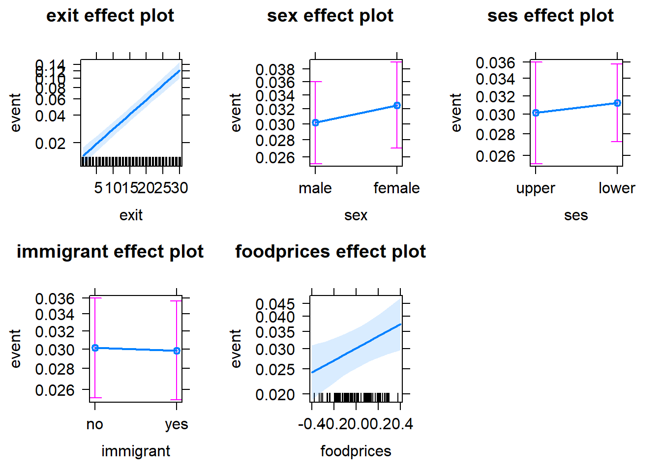
Setting sexfemale = 0 means that the reference level of the sex variable is set to 0 (=male); seslower = 0 means that the reference level of the ses variable is set to 0 (=upper); immigrantyes = 0 means that the reference level of the immigrant variable is set to 0 (=no).
6. Model Evaluation: Goodness of Fit
We introduce here some common tests that we can use to examine the goodness-of-fit of a discrete-time survival model, including the likelihood ratio test, Akaike information criterion (AIC) and deviance residuals.
6.1. Likelihood Ratio Test
A model has a better fit to the data if the model, compared with a model with fewer predictors, demonstrates an improvement in the fit. This is performed using the likelihood ratio test, which compares the likelihood of the data under the full model against the likelihood of the data under a model with fewer predictors. Removing predictor variables from a model will almost always make the model fit less well (i.e. a model will have a lower log likelihood), but it is useful to test whether the observed difference in model fit is statistically significant. In this way, the likelihood ratio test can also be used to determine the relevance of (a group of) variables. As an example, we can test whether our full Gompertz model provides a better fit to the data than the baseline Gompertz model, using the likelihood ratio test. This is done via the anova function.
anova(Gompertz_Model_Baseline, Gompertz_Model_Full, test ="Chisq")## Analysis of Deviance Table
##
## Model 1: event ~ exit
## Model 2: event ~ exit + sex + ses + immigrant + foodprices
## Resid. Df Resid. Dev Df Deviance Pr(>Chi)
## 1 22333 6897.5
## 2 22329 6888.9 4 8.6282 0.07109 .
## ---
## Signif. codes: 0 '***' 0.001 '**' 0.01 '*' 0.05 '.' 0.1 ' ' 1As we can see, the difference between the two models is not significant at 5% level. Therefore, the inclusion of all of the additional predictors (ses, sex, immigrant and foodprices) does not provide a significantly better fit to the data.
6.2. AIC
The Akaike information criterion (AIC) is another measure for model selection. Different from the likelihood ratio test, the calculation of AIC not only regards the goodness of fit of a model, but also takes into account the simplicity of the model. In this way, AIC deals with the trade-off between goodness of fit and complexity of the model, and as a result, disencourages overfitting. A smaller AIC is preferred.
Gompertz_Model_Full$aic## [1] 6900.877Gompertz_Model_Baseline$aic## [1] 6901.505The two models have extremely similar AIC scores, suggesting that their model fit performances are not well differentiated from each other.
6.3. Deviance Residuals
Deviance residuals of a discrete-time survival model can be used to examine the fit of a model on a case-by-case manner. The deviance residual for each individual \(i\) at time \(s\) is calculated via the following formula:
\[DevRes_{is} = \begin{cases}-\sqrt{-2log(1-\hat{h}_{is})} & y_{is} = 0\\\sqrt{-2log(\hat{h}_{is})} & y_{is} = 1\end{cases}\] From the formula we can see that the deviance residual is positive only if, and when, the event occurs. In contrast, deviance residuals are negative in all the time periods before event occurrence and remain negative in the final period for people who have not experienced the target event.
Unlike regular residuals, with deviance residuals we do not examine their distribution nor plot them versus predicted outcome or observed predictor values. We eschew such displays because they will manifest uninformative deterministic patterns. Instead, we examine deviance residuals on a case-by-case basis, generally through the use of index plots: sequential plots by case ID. When examining index plots like these, we look for extreme observations, namely person-period records with extraordinarily large residuals. Large residuals suggest person-period records with poor model fit.
Below we calculate the deviance residuals of the Gompertz full model and make the index plot:
Data_DevResid <- tibble(Pred_Haz = predict(Gompertz_Model_Full, type = "response"),
       Event = pull(Scania_PersonPeriod_Train, event),
       ID = pull(Scania_PersonPeriod_Train, id)) %>%
  mutate(DevRes = if_else(Event == 0,
                          -sqrt(-2*log(1-Pred_Haz)),
                          sqrt(-2*log(Pred_Haz))))
Data_DevResid %>%
  ggplot(aes(x = ID, y = DevRes)) +
  geom_point()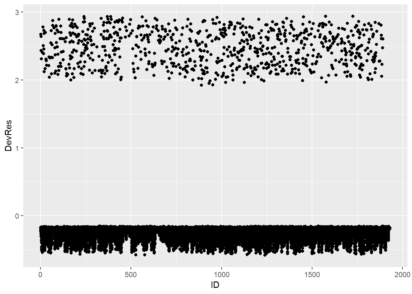
We see no substantially large and outlying residuals (>3 or <-3). However, we also notice that the deviance residiuals of the cases with event occurring are concentrated between 2 and 3, which are relatively far away from 0. In contrast, the cases without event occurring have residuals that are close to 0. This indicates that the model does not provide a good fit to the cases with event occurring.
7. Model Evaluation: Predictive Performance
We have considered several methods for assessing the goodness-of-fit of a discrete-time survival model. They provide information about whether a model is well calibrated. In addition to assessing goodness-of-fit, it is often also our interest to measure the performance of a model with regards to predicting survival or hazards of future observations. We introduce here two such methods: predictive deviance and prediction error curves and apply them to the test data.
7.1. Predictive Deviance
The formula for predictive deviance is as follows:
\[PD = -2 * (\sum_{i=1}^n\sum_{s=1}^{t_{i}} y_{is}\log (\hat{h}_{is}) + (1-y_{is})\log (1-\hat{h}_{is}))\]
The predictive deviance score for the full Gompertz model is computed via the following codes.
#observed hazards
Obs_Haz <- pull(Scania_PersonPeriod_Test, event)

#predicted hazards
Pred_Haz_Full <- predict(Gompertz_Model_Full, Scania_PersonPeriod_Test, type = "response")

#predictive deviance
Pred_Dev_Full <- tibble(obs = Obs_Haz, pred = Pred_Haz_Full) %>%
  mutate(dev = obs*log(pred) + (1-obs)*log(1-pred)) %>%
  summarise(deviance = -2*sum(dev))%>%
  pull(deviance)

Pred_Dev_Full
## [1] 1878.409We get a predictive deviance score of 1878.409 for the full model. This score itself is not informative, unless it is compared with the score of another model (based on the same data). We can calculate the predictive deviance score of the baseline Gompertz model.
#observed hazards
Obs_Haz <- pull(Scania_PersonPeriod_Test, event)

#predicted hazards
Pred_Haz_Baseline <- predict(Gompertz_Model_Baseline, Scania_PersonPeriod_Test, type = "response")

#predictive deviance
Pred_Dev_Baseline <- tibble(obs = Obs_Haz, pred = Pred_Haz_Baseline) %>%
  mutate(dev = obs*log(pred) + (1-obs)*log(1-pred)) %>%
  summarise(deviance = -2*sum(dev))%>%
  pull(deviance)

Pred_Dev_Baseline
## [1] 1872.052With the slightly smaller predictive deviance score, the baseline model predicts future observations better than does the full model. This suggests that the full model likely overfits the data.
7.2. Prediction Error Curves
Prediction Error (PE) curves (\(PE(t)\)) are a time-dependent measure of prediction error based on the squared distance between the predicted individual survival functions \(\hat{S}_{is} = \prod_{s=1}^t (1-\hat{h}_{is})\), and the corresponding observed survival functions \(\tilde{S}_{is} = I(s < T_{i})\), where \(I(.)\) denotes the indicator function, such that the observed survival functions are equal to 1 as long as an observation is still alive and become 0 after the event of interest has occurred. For each time point \(s\) under consideration, the PE curves measure the deviation of what we observe (i.e., \(\tilde{S}_{is}\)) from what is predicted from a statistical model (i.e., \(\hat{S}_{is}\)). The PE curves in addition use inverse probability of censoring weights to account for biases due to censoring. The PE curve becomes small if the predicted survival functions agree closely with the observed survival functions. A well-predicting survival model should result in PE values that are smaller than 0.25 for all \(s\). This is because 0.25 corresponds to the value of the PE curve obtained from a non-informative model with \(\hat{S}_{is} = 0.5\) for all time points.
To calculate PE curves, we can borrow the predErrDiscShort function from the discSurv package. See below how to use the function to calculate the PE curves for the full model. Note that the predErrDiscShort function may take a while (up to several minutes) to run.
#calculate 1 - predicted hazards
OneMinusPredHaz <- 1 - predict(Gompertz_Model_Full,
                               newdata = Scania_PersonPeriod_Test,
                               type = "response")
#calculate individual predicted survival curves
PredSurv <- aggregate(formula = OneMinusPredHaz ~ id,
                      data = Scania_PersonPeriod_Test,
                      FUN=cumprod)

#PE curves for all the 30 time points in the data
PredErrCurve <- predErrDiscShort(timepoints = 1:30,
                                 estSurvList = PredSurv[[2]], #survival curves
                                 newTime = Scania_Person_Test$exit, #time points in the test set
                                 newEvent = Scania_Person_Test$event, #event in the test set
                                 trainTime = Scania_Person_Train$exit, #time points in the training set
                                 trainEvent = Scania_Person_Train$event) #event in the training set
#plot the PE curve
tibble(PE = PredErrCurve$Output$predErr) %>%
  mutate(exit = row_number()) %>%
  ggplot(aes(y = PE, x = exit)) +
  geom_point() +
  geom_line(lty = "dashed") +
  geom_hline(yintercept = 0.25)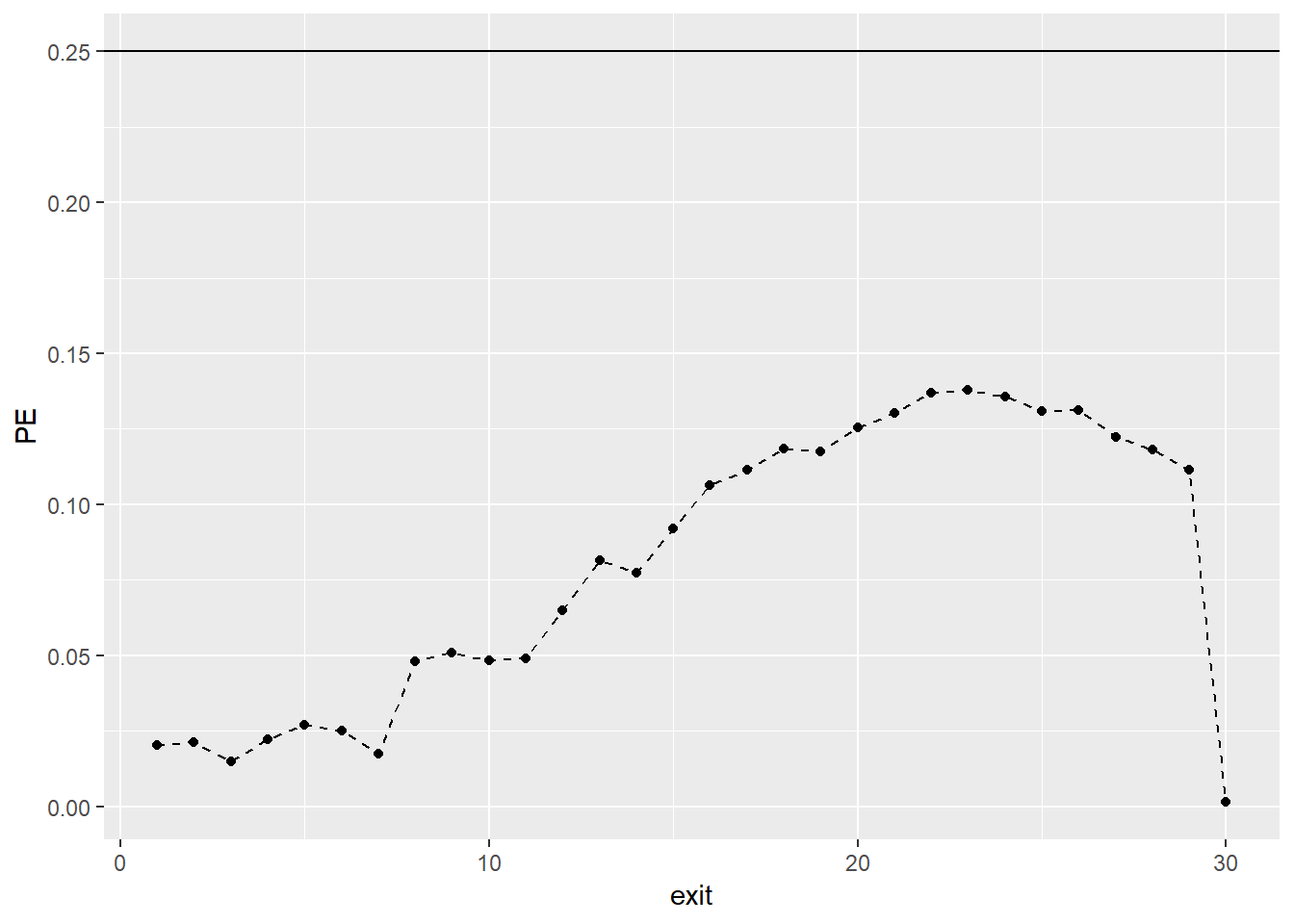
As we can see, all points of the curve stay consistently well below the cut-off value of 0.25. Therefore, the Gompertz full model predicts future survival substantially better than chance. Of course, we can also compare PE curves from competing models.
8. Multilevel Discrete-Time Survival Analysis
In regression modelling, we try to include all relevant predictors. However, most often we have only access to a limited number of potentially influential variables. Because of this, part of the heterogeneity in the population remains unobserved. Unobserved heterogeneity can cause severe problems to especially survival modelling. For instance, with substantial unobserved heterogeneity, the parameter effects that we observe in the model only apply on the population level, but not on the individual level. Multilevel modelling helps to mitigate this issue. The most basic application of multilevel modelling in survival analysis is the so-called basic frailty model, where we assume that every individual has its own hazard function. We do so by introducing a random intercept term.
In R, we can use the lme4 package to specify multilevel discrete-time survival regression models. See below as an example of how to specify the basic frailty model. For a detailed introduction to multilevel models with lme4, check out the tutorial Lme4 introduction (frequentist).
Model_Multi <- glmer(formula = event ~ exit + sex + ses + immigrant + foodprices + (1|id),
                     family = binomial(cloglog),
                     data = Scania_PersonPeriod_Train,
                     control = glmerControl(optimizer = "bobyqa",
                                            optCtrl = list(maxfun = 2e5)))
## boundary (singular) fit: see ?isSingular#you can normally ignore the control argument. It is used here to increase the maximum iteration.
summary(Model_Multi)## Generalized linear mixed model fit by maximum likelihood (Laplace
## Approximation) [glmerMod]
## Family: binomial ( cloglog )
## Formula: event ~ exit + sex + ses + immigrant + foodprices + (1 | id)
## Data: Scania_PersonPeriod_Train
## Control:
## glmerControl(optimizer = "bobyqa", optCtrl = list(maxfun = 2e+05))
##
## AIC BIC logLik deviance df.resid
## 6902.9 6959.0 -3444.4 6888.9 22328
##
## Scaled residuals:
## Min 1Q Median 3Q Max
## -0.4297 -0.2186 -0.1678 -0.1393 8.5971
##
## Random effects:
## Groups Name Variance Std.Dev.
## id (Intercept) 0 0
## Number of obs: 22335, groups: id, 1545
##
## Fixed effects:
## Estimate Std. Error z value Pr(>|z|)
## (Intercept) -4.306098 0.112043 -38.433 < 2e-16 ***
## exit 0.075387 0.004212 17.900 < 2e-16 ***
## sexfemale 0.077144 0.069079 1.117 0.26410
## seslower 0.036177 0.086375 0.419 0.67533
## immigrantyes -0.009161 0.069518 -0.132 0.89516
## foodprices 0.549623 0.206695 2.659 0.00784 **
## ---
## Signif. codes: 0 '***' 0.001 '**' 0.01 '*' 0.05 '.' 0.1 ' ' 1
##
## Correlation of Fixed Effects:
## (Intr) exit sexfml seslwr immgrn
## exit -0.604
## sexfemale -0.254 0.001
## seslower -0.575 0.017 -0.099
## immigrantys -0.331 0.026 -0.010 -0.057
## foodprices -0.039 0.004 -0.005 0.007 0.007
## convergence code: 0
## boundary (singular) fit: see ?isSingularNote that the basic frailty model has a negative log-likelihood of -3444.4 and an AIC of 6902.9. In comparison, the previous Gompertz model without the person-level frailty term has a negative log-likelihood of -3444.438 and AIC of 6900.877. The almost identical log-likelihood scores and AIC scores between the two models suggests that there is no need for a frailty model.
This tutorial does not delve deeper into multilevel extensions of discrete-time survival regression. For this specific topic, please see Chapter 9 of Modeling Discrete Time-to-Event Data by Tutz & Schmid (2016). For more multilevel modelling in general, check out Multilevel analysis: Techniques and applications. For introduction to GLM or multilevel modelling in R, see the relevant tutorials on Online Stats Training.
9. Bayesian Discrete-Time Survival Analysis
If you would like to work with the Bayesian framework for discrete-time survival analysis (multilevel or not), you can use the brms package in R. As discrete-time regression analysis uses the glm framework, if you know how to use the brms package to set up a Bayesian generalised linear model, you are good to go. For this, check out the relevant tutorials on Online Stats Training, such as BRMS getting started and Intro to Bayesian (Multilevel) Generalised Linear Models (GLM) in R with brms. We also recommend that you follow the WAMBS-checklist if you do use the Bayesian approach in your research.
Below is an example of how to use the brms package to set up the previous Gompertz full model. The model estimates will be almost the same as the model fitted by glm. Kindly note that running a model with brms takes quite some time (~minutes). Feel free to run it by yourself.
Bayes_Model <- brm(formula = event ~ exit + sex + ses + immigrant + foodprices,
                   data = Scania_PersonPeriod_Train,
                   family = bernoulli(link = "cloglog"),
                   warmup = 500,
                   iter = 2000,
                   chains = 2,
                   inits= "0",
                   cores=2,
                   seed = 123)
Bayes_Model
Reference
Bates, D., Maechler, M., Bolker, B., & Walker, S. (2015). Fitting Linear Mixed-Effects Models Using lme4. Journal of Statistical Software, 67(1), 1-48. doi:10.18637/jss.v067.i01
Broström, G. (2018). eha: Event History Analysis. R package version 2.6.0. https://CRAN.R-project.org/package=eha
Bürkner, P. (2017). brms: An R Package for Bayesian Multilevel Models Using Stan. Journal of Statistical Software, 80(1), 1-28. doi:10.18637/jss.v080.i01
Fox, J. (2003). Effect Displays in R for Generalised Linear Models. Journal of Statistical Software, 8(15), 1-27. http://www.jstatsoft.org/v08/i15/
Long, JA. (2019). jtools: Analysis and Presentation of Social Scientific Data. R package version 2.0.1, https://cran.r-project.org/package=jtools
Tutz, G., & Schmid, M. (2016). Modeling Discrete Time-to-Event Data (1st ed.). Springer New York. https://doi.org/10.1007/978-3-319-28158-2
Welchowski, T., & Schmid, M (2018). discSurv: Discrete Time Survival Analysis. R package version 1.3.4. https://CRAN.R-project.org/package=discSurv
Wickham, H. (2017). tidyverse: Easily Install and Load the ‘Tidyverse’. R package version 1.2.1. https://CRAN.R-project.org/package=tidyverse