Intro to Frequentist (Multilevel) Generalised Linear Models (GLM) in R with glm and lme4
Qixiang Fang and Rens van de Schoot
Last modified: date: 14 October 2019
This tutorial provides the reader with a basic introduction to genearlised linear models (GLM) using the frequentist approach. Specifically, this tutorial focuses on the use of logistic regression in both binary-outcome and count/porportion-outcome scenarios, and the respective approaches to model evaluation. The tutorial uses the Thai Educational Data example in Chapter 6 of the book Multilevel analysis: Techniques and applications. Furthermore, the tutorial briefly demonstrates the multilevel extension of GLM models with the lme4 package in R. Lastly, more distributions and link functions in the GLM framework are discussed.
This tutorial follows this structure:
1. Preparation;
2. Introduction to GLM;
3. Thai Educational Data;
4. Data Preparation;
5. Binary (Bernoulli) Logistic Regression;
6. Binomial Logistic Regression;
7. Multilevel Logistic Regression;
8. Other Family and Link Functions.
Note that this tutorial is meant for beginners and therefore does not delve into technical details and complex models. For a detailed introduction into frequentist multilevel models, see this LME4 Tutorial. For an extensive overview of GLM models, see here. The Bayesian version of this tutorial can also be found here.
This tutorial expects:
– Installation of R packages lme4 for multilevel modelling (this tutorial uses version 1.1-18-1);
– Installation of R package tidyverse for data manipulation and plotting with ggplot2;
– Installation of R package haven for reading sav format data;
– Installation of R package jtools for handling of model summaries;
– Installation of R package ggstance for visualisation purposes;
– Installation of R package ROCR for calculating area under the curve (AUC);
– Installation of R package sjstats for calculating intra-class correlation (ICC). Remember to install version 0.17.5 (using the command install_version("sjstats", version = "0.17.5") after loading the package devtools, because the latest version of sjstats does not support the ICC function anymore);
– Installation of R package effects for plotting parameter effects;
– Basic knowledge of hypothesis testing and statistical inference;
– Basic knowledge of correlation and regression;
– Basic knowledge of coding in R;
– Basic knowledge of plotting and data manipulation with tidyverse.
2. Introduction to Genearlised Linear Models (GLM)
If you are already familar with generalised linear models (GLM), you can proceed to the next section. Otherwise, click “Read More” to learn about GLM.
Recall that in a linear regression model, the object is to model the expected value of a continuous variable, \(Y\), as a linear function of the predictor, \(\eta = X\beta\). The model structure is thus: \(E(Y) = X\beta + e\), where \(e\) refers to the residual error term. The linear regression model assumes that \(Y\) is continuous and comes from a normal distribution, that \(e\) is normally distributed and that the relationship between the linear predictor \(\eta\) and the expected outcome \(E(Y)\) is strictly linear. However, these assumptions are easily violated in many real world data examples, such as those with binary or proportional outcome variables and those with non-linear relationships between the predictors and the outcome variable. In these scenarios where linear regression models are clearly inappropriate, generalised linear models (GLM) are needed.
The GLM is the genearlised version of linear regression that allows for deviations from the assumptions underlying linear regression. The GLM generalises linear regression by assuming the dependent variable \(Y\) to be generated from any particular distribution in an exponential family (a large class of probability distributions that includes the normal, binomial, Poisson and gamma distributions, among others). In this way, the distribution of \(Y\) does not necessarily have to be normal. In addition, the GLM allows the linear predictor \(\eta\) to be connected to the expected value of the outcome variable, \(E(Y)\), via a link function \(g(.)\). The outcome variable, \(Y\), therefore, depends on \(\eta\) through \(E(Y) = g^{-1}(\eta) = g^{-1}(X\beta)\). In this way, the model does not assume a linear relationship between \(E(Y)\) and \(\eta\); instead, the model assumes a linear relationship between \(E(Y)\) and the transformed \(g^{-1}(\eta)\).
This tutorial focuses on the probably most popular example of GLM: logistic regression. Logistic regression has two variants, the well-known binary logistic regression that is used to model binary outcomes (1 or 0; “yes” or “no”), and the less-known binomial logistic regression suited to model count/proportion data.
Binary logistic regression assumes that \(Y\) comes from a Bernoulli distribution, where \(Y\) only takes a value of 1 (target event) or 0 (non-target event). Binary logistic regression connects \(E(Y)\) and \(\eta\) via the logit link \(\eta = logit(\pi) = log(\pi/(1-\pi))\), where \(\pi\) refers to the probability of the target event (\(Y = 1\)).
Binomial logistic regression, in contrast, assumes a binomial distribution underlying \(Y\), where \(Y\) is interpreted as the number of target events, can take on any non-negative integer value and is binomially distributed with regards to \(n\) number of trials and \(\pi\) probability of the target event. The link function is the same as that of binary logistic regression.
The next section details the exampler data (Thai Educational Data) in this tutorial, followed by the demonstration of the use of both binary and binomial logistic regression.
3. Thai Educational Data
The data used in this tutorial is the Thai Eduational Data that is also used as an example in Chapter 6 of Multilevel analysis: Techniques and applications. The data can be downloaded from here.
The data stems from a national survey of primary education in Thailand (Raudenbush & Bhumirat, 1992). Each row in the data refers to a pupil. The outcome variable REPEAT is a dichotomous variable indicating whether a pupil has repeated a grade during primary education. The SCHOOLID variable indicates the school of a pupil. The person-level predictors include: SEX (0 = female, 1 = male) and PPED (having had preschool education, 0 = no, 1 = yes). The school-level is MSESC, representing school mean SES (socio-economic status) scores.
The main research questions that this tutorial seeks to answer using the Thai Educational Data are:
- Ignoring the clustering structure of the data, what are the effects of gender and preschool education on whether a pupil repeats a grade?
- Ignoring the clustering structure of the data, what is the effect of school mean SES on the proportion of pupil repeating a grade?
- Considering the clustering structure of the data, what are the effects of gender, preschool education and school mean SES on whether a pupil repeats a grade?
These three questions are answered by using these following models, respectively: binary logistic regressioin; binomial logistic regression; multilevel binary logistic regression.
4. Data Preparation
4.1. Load necessary packages
# if you dont have these packages installed yet, please use the install.packages("package_name") command.
library(lme4) # for multilevel models
library(tidyverse) # for data manipulation and plots
library(haven) #for reading sav data
library(sjstats) #for calculating intra-class correlation (ICC)
library(effects) #for plotting parameter effects
library(jtools) #for transformaing model summaries
library(ROCR) #for calculating area under the curve (AUC) statistics
4.2. Import Data
ThaiEdu_Raw <- read_sav("https://github.com/MultiLevelAnalysis/Datasets-third-edition-Multilevel-book/blob/master/chapter%206/Thaieduc/thaieduc.sav?raw=true")
head(ThaiEdu_Raw)
## # A tibble: 6 x 5
## SCHOOLID SEX PPED REPEAT MSESC
## <dbl> <dbl+lbl> <dbl+lbl> <dbl+lbl> <dbl>
## 1 10101 0 [girl] 1 [yes] 0 [no] NA
## 2 10101 0 [girl] 1 [yes] 0 [no] NA
## 3 10101 0 [girl] 1 [yes] 0 [no] NA
## 4 10101 0 [girl] 1 [yes] 0 [no] NA
## 5 10101 0 [girl] 1 [yes] 0 [no] NA
## 6 10101 0 [girl] 1 [yes] 0 [no] NAAlternatively, you can download the data directly from here and import it locally.
4.3. Data Processing
ThaiEdu_New <- ThaiEdu_Raw %>%
  mutate(SCHOOLID = factor(SCHOOLID),
         SEX = if_else(SEX == 0, "girl", "boy"),
         SEX = factor(SEX, levels = c("girl", "boy")),
         PPED = if_else(PPED == 0, "no", "yes"),
         PPED = factor(PPED, levels = c("no", "yes")))

head(ThaiEdu_New)
## # A tibble: 6 x 5
## SCHOOLID SEX PPED REPEAT MSESC
## <fct> <fct> <fct> <dbl+lbl> <dbl>
## 1 10101 girl yes 0 [no] NA
## 2 10101 girl yes 0 [no] NA
## 3 10101 girl yes 0 [no] NA
## 4 10101 girl yes 0 [no] NA
## 5 10101 girl yes 0 [no] NA
## 6 10101 girl yes 0 [no] NA4.4. Inspect Missing Data
ThaiEdu_New %>%
  summarise_each(list(~sum(is.na(.)))) %>%
  gather()
## # A tibble: 5 x 2
## key value
## <chr> <int>
## 1 SCHOOLID 0
## 2 SEX 0
## 3 PPED 0
## 4 REPEAT 0
## 5 MSESC 1066The data has 1066 observations missing for the MSESC variable. The treatment of missing data is a complicated topic on its own. For the sake of convenience, we simply list-wise delete the cases with missing data in this tutorial.
ThaiEdu_New <- ThaiEdu_New %>%
  filter(!is.na(MSESC))
5. Binary Logistic Regression
5.1. Explore Data: number of REPEAT by SEX and PPED
ThaiEdu_New %>%
  group_by(SEX) %>%
  summarise(REPEAT = sum(REPEAT))
## # A tibble: 2 x 2
## SEX REPEAT
## <fct> <dbl>
## 1 girl 428
## 2 boy 639ThaiEdu_New %>%
group_by(PPED) %>%
summarise(REPEAT = sum(REPEAT))## # A tibble: 2 x 2
## PPED REPEAT
## <fct> <dbl>
## 1 no 673
## 2 yes 394It seems that the number of pupils who repeated a grade differs quite a bit between the two genders, with more male pupils having to repeat a grade. More pupils who did not have preschool education repeated a grade. This observation suggests that SEX and PPED might be predictive of REPEAT.
5.2. Fit a Binary Logistic Regression Model
R has the base package installed by default, which includes the glm function that runs GLM. The arguments for glm are similar to those for lm: formula and data. However, glm requires an additional argument: family, which specifies the assumed distribution of the outcome variable; within family we also need to specify the link function. The default of family is gaussian(link = "identity"), which leads to a linear model that is equivalent to a model specified by lm. In the case of binary logistic regression, glm requires that we specify a binomial distribution with the logit link, namely family = binomial(link = "logit").
Model_Binary <- glm(formula = REPEAT ~ SEX + PPED,
                    family = binomial(link = "logit"),
                    data = ThaiEdu_New)
summary(Model_Binary)
##
## Call:
## glm(formula = REPEAT ~ SEX + PPED, family = binomial(link = "logit"),
## data = ThaiEdu_New)
##
## Deviance Residuals:
## Min 1Q Median 3Q Max
## -0.6844 -0.5630 -0.5170 -0.4218 2.2199
##
## Coefficients:
## Estimate Std. Error z value Pr(>|z|)
## (Intercept) -1.76195 0.05798 -30.387 < 2e-16 ***
## SEXboy 0.42983 0.06760 6.358 2.04e-10 ***
## PPEDyes -0.61298 0.06833 -8.971 < 2e-16 ***
## ---
## Signif. codes: 0 '***' 0.001 '**' 0.01 '*' 0.05 '.' 0.1 ' ' 1
##
## (Dispersion parameter for binomial family taken to be 1)
##
## Null deviance: 6140.8 on 7515 degrees of freedom
## Residual deviance: 6016.2 on 7513 degrees of freedom
## AIC: 6022.2
##
## Number of Fisher Scoring iterations: 45.3. Interpretation
From the summary output above, we can see that SEX positively and significantly predicts a pupil’s probability of repeating a grade, while PPED negatively and significantly so. Specifically, in comparison to being a girl, being a boy is more likely to repeat a grade. Having previous schooling is less likely to result in repeating a grade.
To interpret the value of the parameter estimates, we need to exponentiate the estimates. The summ function from the jtools packages provides an easy to do so for any model fitted by glm. See below.
summ(Model_Binary, exp = T) # set "exp = T" to show esponentiated estimates; if you need standardised estimaets, set "scale = T"## MODEL INFO:
## Observations: 7516
## Dependent Variable: REPEAT
## Type: Generalized linear model
## Family: binomial
## Link function: logit
##
## MODEL FIT:
## <U+03C7>²(2) = 124.55, p = 0.00
## Pseudo-R² (Cragg-Uhler) = 0.03
## Pseudo-R² (McFadden) = 0.02
## AIC = 6022.21, BIC = 6042.98
##
## Standard errors: MLE
##
## | | exp(Est.)| 2.5%| 97.5%| z val.| p|
## |:-----------|---------:|----:|-----:|------:|----:|
## |(Intercept) | 0.17| 0.15| 0.19| -30.39| 0.00|
## |SEXboy | 1.54| 1.35| 1.75| 6.36| 0.00|
## |PPEDyes | 0.54| 0.47| 0.62| -8.97| 0.00|Note that the interpretation of the parameter estimates is linked to the odds rather than probabilities. The definition of odds is: P(event occurring)/P(event not occurring). In this analysis, assuming everything else stays the same, being a boy increases the odds of repeating a grade by 54%, in comparison to being a girl; having preschool education lowers the odds of repeating a grade by (1 – 0.54)% = 46%, in comparison to not having preschool education, assuming everything else stays constant.
5.4. Visualisation of Parameter Effects
To make the interpretation of the parameter effects even easier, we can use the allEffects function from the effects package to visualise the parameter effects. See below.
plot(allEffects(Model_Binary))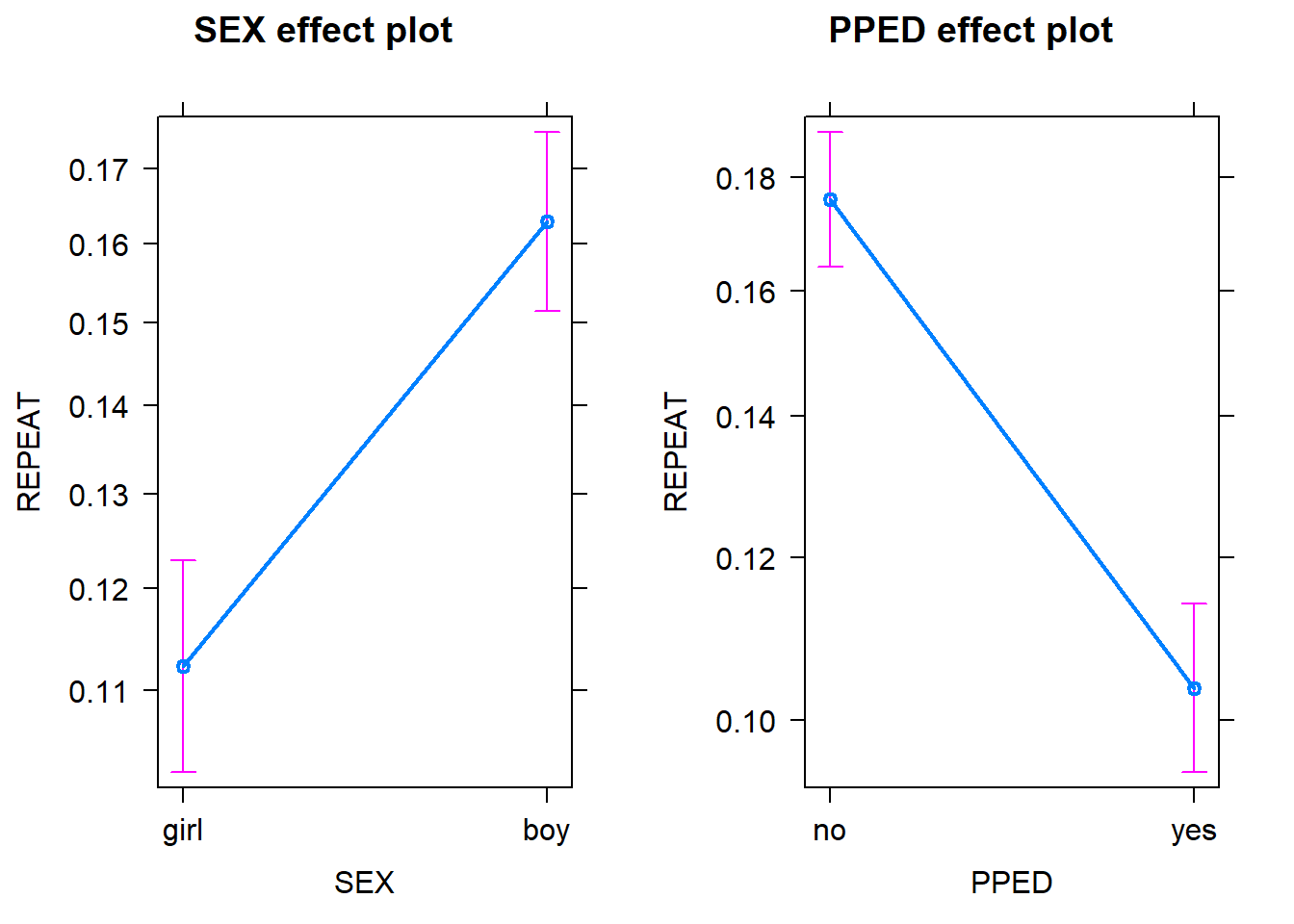
Note that in both plots, the y scale refers to the probability of repeating a grade rather than the odds. Probabilities are more interpretable than odds. The probability scores for each variable are calculated by assuming that the other variables in the model are constant and take on their average values. As we can see, assuming that a pupil has an average preschool education, being a boy has a higher probability (~0.16) of repeating a grade than being a girl ~0.11). Likewise, assuming that a pupil has an average gender, having preschool education has a lower probability (~0.11) of repeating a grade than not having preschool education (~0.18). Note that in both plots the confidence intervals for the estimates are also included to give us some idea of the uncertainties of the estimates.
Note that the notion of average preschool education and gender may sound strange, given they are categorical variables (i.e. factors). If you are not comfortable with the idea of assuming an average factor, you can specify your intended factor level as the reference point, by using the fixed.predictors = list(given.values = ...) argument in the allEffects function. See below:
plot(allEffects(Model_Binary, fixed.predictors = list(given.values=c(SEXboy=0, PPEDyes = 0))))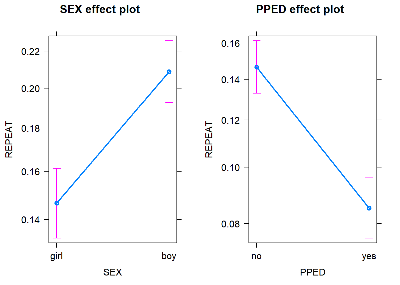
Setting SEXboy = 0 means that for the PPED effect plot, the reference level of the SEX variable is set to 0; PPEDyes = 0 results in the 0 being the reference level of the PPED variable in the SEX effect plot.
Therefore, as the two plots above show, assuming that a pupil has no preschool education, being a boy has a higher probability (~0.20) of repeating a grade than being a girl ~0.14); assuming that a pupil is female, having preschool education has a lower probability (~0.09) of repeating a grade than not having preschool education (~0.15).
5.5. Model Evaluation: Goodness of Fit
There are different ways to evaluate the goodness of fit of a logistic regression model.
5.5.1. Likelihood ratio test
A logistic regression model has a better fit to the data if the model, compared with a model with fewer predictors, demonstrates an improvement in the fit. This is performed using the likelihood ratio test, which compares the likelihood of the data under the full model against the likelihood of the data under a model with fewer predictors. Removing predictor variables from a model will almost always make the model fit less well (i.e. a model will have a lower log likelihood), but it is useful to test whether the observed difference in model fit is statistically significant.
#specify a model with only the `SEX` variable
Model_Binary_Test <- glm(formula = REPEAT ~ SEX,
                         family = binomial(link = "logit"),
                         data = ThaiEdu_New)

#use the `anova()` function to run the likelihood ratio test
anova(Model_Binary_Test, Model_Binary, test ="Chisq")
## Analysis of Deviance Table
##
## Model 1: REPEAT ~ SEX
## Model 2: REPEAT ~ SEX + PPED
## Resid. Df Resid. Dev Df Deviance Pr(>Chi)
## 1 7514 6099.1
## 2 7513 6016.2 1 82.941 < 2.2e-16 ***
## ---
## Signif. codes: 0 '***' 0.001 '**' 0.01 '*' 0.05 '.' 0.1 ' ' 1As we can see, the model with both SEX and PPED predictors provide a significantly better fit to the data than does the model with only the SEX variable. Note that this method can also be used to determine whether it is necessary to include one or a group of variables.
5.5.2. AIC
The Akaike information criterion (AIC) is another measure for model selection. Different from the likelihood ratio test, the calculation of AIC not only regards the goodness of fit of a model, but also takes into account the simplicity of the model. In this way, AIC deals with the trade-off between goodness of fit and complexity of the model, and as a result, disencourages overfitting. A smaller AIC is preferred.
Model_Binary_Test$aic## [1] 6103.148Model_Binary$aic## [1] 6022.207With a smaller AIC value, the model with both SEX and PPED predictors is preferred to the one with just the SEX predictor.
5.5.3. Correct Classification Rate
The percentage of correct classification is another useful measure to see how well the model fits the data.
#use the `predict()` function to calculate the predicted probabilities of pupils in the original data from the fitted model
Pred <- predict(Model_Binary, type = "response")
Pred <- if_else(Pred > 0.5, 1, 0)
ConfusionMatrix <- table(Pred, pull(ThaiEdu_New, REPEAT)) #`pull` results in a vector
#correct classification rate
sum(diag(ConfusionMatrix))/sum(ConfusionMatrix)
## [1] 0.8580362ConfusionMatrix##
## Pred 0 1
## 0 6449 1067We can see that the model correctly classifies 85.8% of all the observations. However, a closer look reveals that the model predicts all of the observations to belong to class “0”, meaning that all pupils are predicted not to repeat a grade. Given that the majority category of the REPEAT variable is 0 (No), the model does not perform better in classification than simply assigning all observations to the majority class 0 (No).
5.5.4. AUC (area under the curve).
An alternative to using correct classification rate is the Area under the Curve (AUC) measure. The AUC measures discrimination, that is, the ability of the test to correctly classify those with and without the target response. In the current data, the target response is repeating a grade. We randomly pick one pupil from the “repeating a grade” group and one from the “not repeating a grade” group. The pupil with the higher predicted probability should be the one from the “repeating a grade” group. The AUC is the percentage of randomly drawn pairs for which this is true. This procedure sets AUC apart from the correct classification rate because the AUC is not dependent on the imblance of the proportions of classes in the outcome variable. A value of 0.50 means that the model does not classify better than chance. A good model should have an AUC score much higher than 0.50 (preferably higher than 0.80).
# Compute AUC for predicting Class with the model
Prob <- predict(Model_Binary, type="response")
Pred <- prediction(Prob, as.vector(pull(ThaiEdu_New, REPEAT)))
AUC <- performance(Pred, measure = "auc")
AUC <- AUC@y.values[[1]]
AUC
## [1] 0.6013622With an AUC score of 0.60, the model does not discriminate well.
6. Binomial Logistic Regression
As mentioned in the beginning, logistic regression can also be used to model count or proportion data. Binary logistic regression assumes that the outcome variable comes from a bernoulli distribution (which is a special case of binomial distributions) where the number of trial \(n\) is 1 and thus the outcome variable can only be 1 or 0. In contrast, binomial logistic regression assumes that the number of the target events follows a binomial distribution with \(n\) trials and probability \(q\). In this way, binomial logistic regression allows the outcome variable to take any non-negative integer value and thus is capable of handling count data.
The Thai Educational Data records information about individual pupils that are clustered within schools. By aggregating the number of pupils who repeated a grade by school, we obtain a new data set where each row represents a school, with information about the proportion of pupils repeating a grade in that school. The MSESC (mean SES score) is also on the school level; therefore, it can be used to predict proportion or count of pupils who repeat a grade in a particular school. See below.
6.1. Tranform Data
ThaiEdu_Prop <- ThaiEdu_New %>%
  group_by(SCHOOLID, MSESC) %>%
  summarise(REPEAT = sum(REPEAT),
            TOTAL = n()) %>%
  ungroup()

head(ThaiEdu_Prop)
## # A tibble: 6 x 4
## SCHOOLID MSESC REPEAT TOTAL
## <fct> <dbl> <dbl> <int>
## 1 10103 0.88 1 17
## 2 10104 0.2 0 29
## 3 10105 -0.07 5 18
## 4 10106 0.47 0 5
## 5 10108 0.76 3 19
## 6 10109 1.06 9 21In this new data set, REPEAT refers to the number of pupils who repeated a grade; TOTAL refers to the total number of students in a particular school.
6.2. Explore data
ThaiEdu_Prop %>%
  ggplot(aes(x = exp(MSESC)/(1+exp(MSESC)), y = REPEAT/TOTAL)) +
  geom_point() +
  geom_smooth(method = "lm")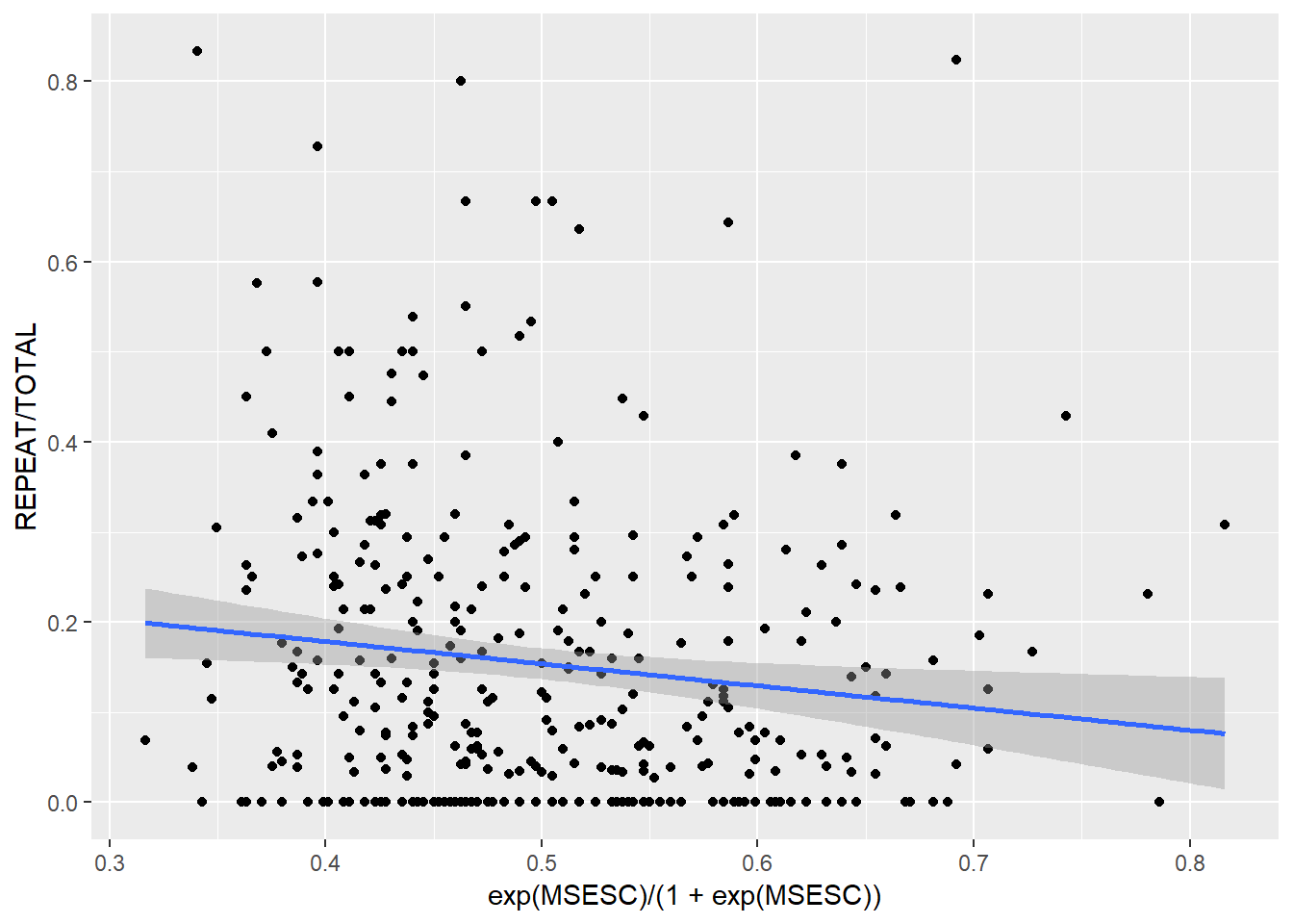
We can see that the proportion of students who repeated a grade is negatively related to the inverse-logit of MSESC. Note that we model the variable MSESC as its inverse-logit because in a binomial regression model, we assume a linear relationship between the inverse-logit of the linear predictor and the outcome (i.e. proportion of events), not linearity between the predictor itself and the outcome.
6.3. Fit a Binomial Logistic Regression Model
To fit a binomial logistic regression model, we also use the glm function. The only difference is in the specification of the outcome variable in the formula. We need to specify both the number of target events (REPEAT) and the number of non-events (TOTAL-REPEAT) and wrap them in cbind().
Model_Prop <- glm(formula = cbind(REPEAT, TOTAL-REPEAT) ~ MSESC,
                  family = binomial(logit),
                  data = ThaiEdu_Prop)

summary(Model_Prop)
##
## Call:
## glm(formula = cbind(REPEAT, TOTAL - REPEAT) ~ MSESC, family = binomial(logit),
## data = ThaiEdu_Prop)
##
## Deviance Residuals:
## Min 1Q Median 3Q Max
## -3.3629 -1.8935 -0.5083 1.1674 6.9494
##
## Coefficients:
## Estimate Std. Error z value Pr(>|z|)
## (Intercept) -1.80434 0.03324 -54.280 < 2e-16 ***
## MSESC -0.43644 0.09164 -4.763 1.91e-06 ***
## ---
## Signif. codes: 0 '***' 0.001 '**' 0.01 '*' 0.05 '.' 0.1 ' ' 1
##
## (Dispersion parameter for binomial family taken to be 1)
##
## Null deviance: 1480.7 on 355 degrees of freedom
## Residual deviance: 1457.3 on 354 degrees of freedom
## AIC: 2192
##
## Number of Fisher Scoring iterations: 56.4. Interpretation
The parameter interpretation in a binomial regression model is the same as that in a binary logistic regression model. We know from the model summary above that the mean SES score of a school is negatively related to the odds of students repeating a grade in that school. To enhance interpretability, we use the summ() function again to calculate the exponentiated coefficient estimate of MSESC. Since MSESC is a continous variable, we can standardise the exponentiated MSESC estimate (by multiplying the original estimate with the SD of the variable, and then then exponentiating the resulting number).
#Note that to use the summ() function for a binomial regression model, we need to make the outcome variable explicit objects:
REPEAT <- pull(filter(ThaiEdu_Prop, !is.na(MSESC)), REPEAT)
TOTAL <- pull(filter(ThaiEdu_Prop, !is.na(MSESC)), TOTAL)
summ(Model_Prop, exp = T, scale = T)
## MODEL INFO:
## Observations: 356
## Dependent Variable: cbind(REPEAT, TOTAL - REPEAT)
## Type: Generalized linear model
## Family: binomial
## Link function: logit
##
## MODEL FIT:
## <U+03C7>²(1) = 23.36, p = 0.00
## Pseudo-R² (Cragg-Uhler) = 0.06
## Pseudo-R² (McFadden) = 0.01
## AIC = 2191.96, BIC = 2199.71
##
## Standard errors: MLE
##
## | | exp(Est.)| 2.5%| 97.5%| z val.| p|
## |:-----------|---------:|----:|-----:|------:|----:|
## |(Intercept) | 0.16| 0.15| 0.18| -54.26| 0.00|
## |MSESC | 0.85| 0.79| 0.91| -4.76| 0.00|
##
## Continuous predictors are mean-centered and scaled by 1 s.d.We can see that with a SD increase in MSESC, the odds of students repeating a grade is lowered by 1 – 85% = 15%.
We can visualise the effect of MSESC.
plot(allEffects(Model_Prop))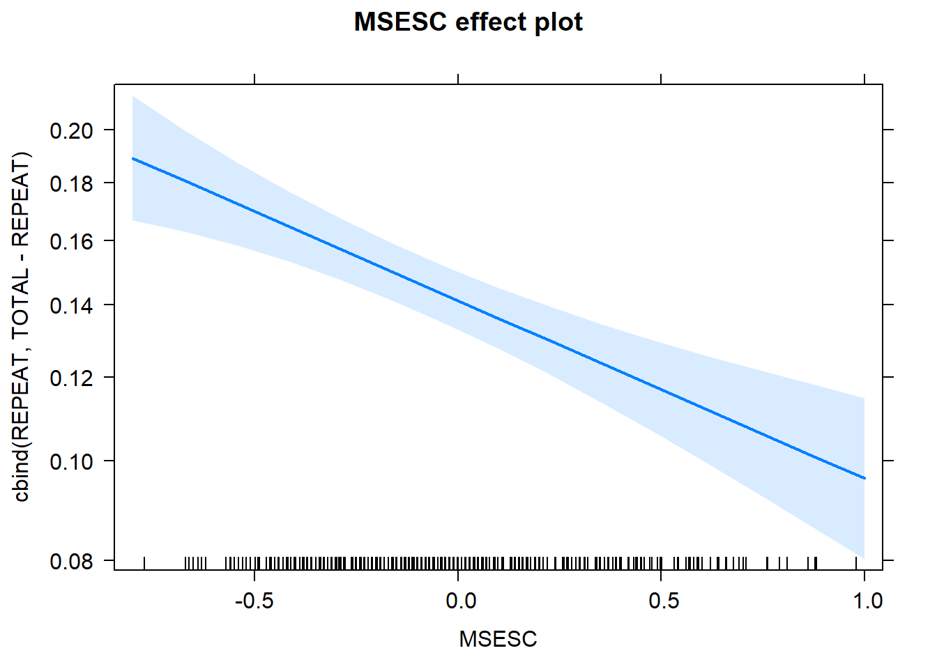
The plot above shows the expected influence of MSESC on the probability of a pupil repeating a grade. Holding everything else constant, as MSESC increases, the probability of a pupil repeating a grade lowers (from 0.19 to 0.10). The blue shaded areas indicate the 95% confidence intervals of the predicted values at each value of MSESC.
7. Multilevel Binary Logistic Regression
The binary logistic regression model introduced earlier is limited to modelling the effects of pupil-level predictors; the binomial logistic regression is limited to modelling the effects of school-level predictors. To incorporate both pupil-level and school-level predictors, we can use multilevel models, specifically, multilevel binary logistic regression. If you are unfamiliar with multilevel models, you can use Multilevel analysis: Techniques and applications for reference and this tutorial for a good introduction to multilevel models with the lme4 package in R.
In addition to the motivation above, there are more reasons to use multilevel models. For instance, as the data are clustered within schools, it is likely that pupils from the same school are more similar to each other than those from other schools. Because of this, in one school, the probability of a pupil repeating a grade may be high, while in another school, low. Furthermore, even the relationship between the outcome (i.e. repeating a grade) and the predictor variabales (e.g. gender, preschool education, SES) may be different across schools. Also note that there are missing values in the MSESC variable. Using multilevel models can appropriately address these issues.
See the following plot as an example. The plot shows the proportions of students repeating a grade across schools. We can see vast differences across schools. Therefore, we may need multilevel models.
ThaiEdu_New %>%
  group_by(SCHOOLID) %>%
  summarise(PROP = sum(REPEAT)/n()) %>%
  plot()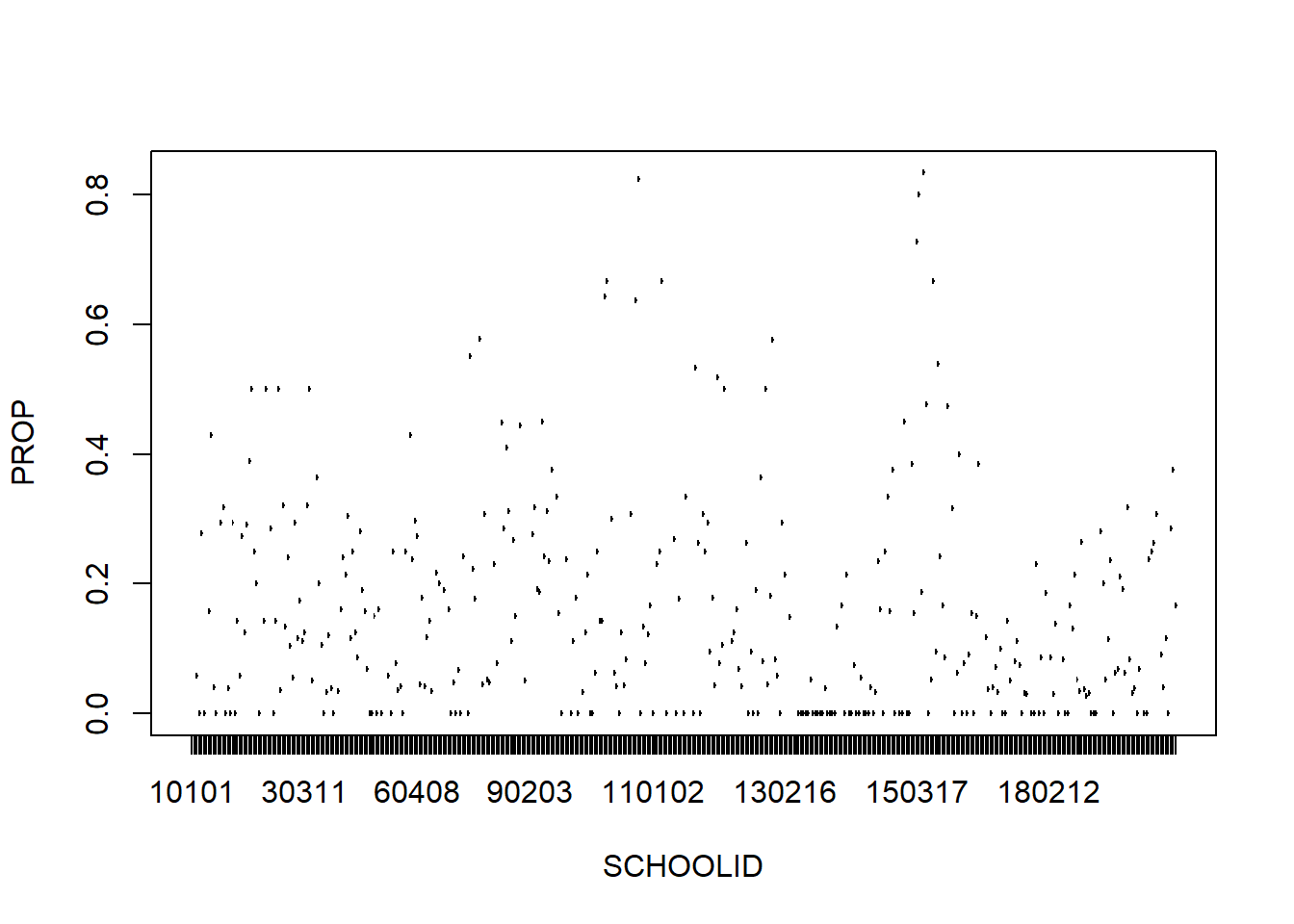
We can also plot the relationship between SEX and REPEAT by SCHOOLID, to see whether the relationship between gender and repeating a grade differs by school.
ThaiEdu_New %>%
  mutate(SEX = if_else(SEX == "boy", 1, 0)) %>%
  ggplot(aes(x = SEX, y = REPEAT, color = as.factor(SCHOOLID))) +
  geom_point(alpha = .1, position = "jitter")+
  geom_smooth(method = "glm", se = F,
              method.args = list(family = "binomial")) +
  theme(legend.position = "none") +
  scale_x_continuous(breaks = c(0, 1)) +
  scale_y_continuous(breaks = c(0, 1))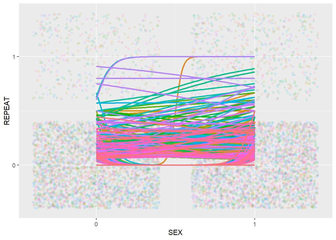
In the plot above, different colors represent different schools. We can see that the relationship between SEX and REPEAT appears to be quite different across schools.
We can make the same plot for PPED and REPEAT.
ThaiEdu_New %>%
  mutate(PPED = if_else(PPED == "yes", 1, 0)) %>%
  ggplot(aes(x = PPED, y = REPEAT, color = as.factor(SCHOOLID))) +
  geom_point(alpha = .1, position = "jitter")+
  geom_smooth(method = "glm", se = F,
              method.args = list(family = "binomial")) +
  theme(legend.position = "none") +
  scale_x_continuous(breaks = c(0, 1)) +
  scale_y_continuous(breaks = c(0, 1))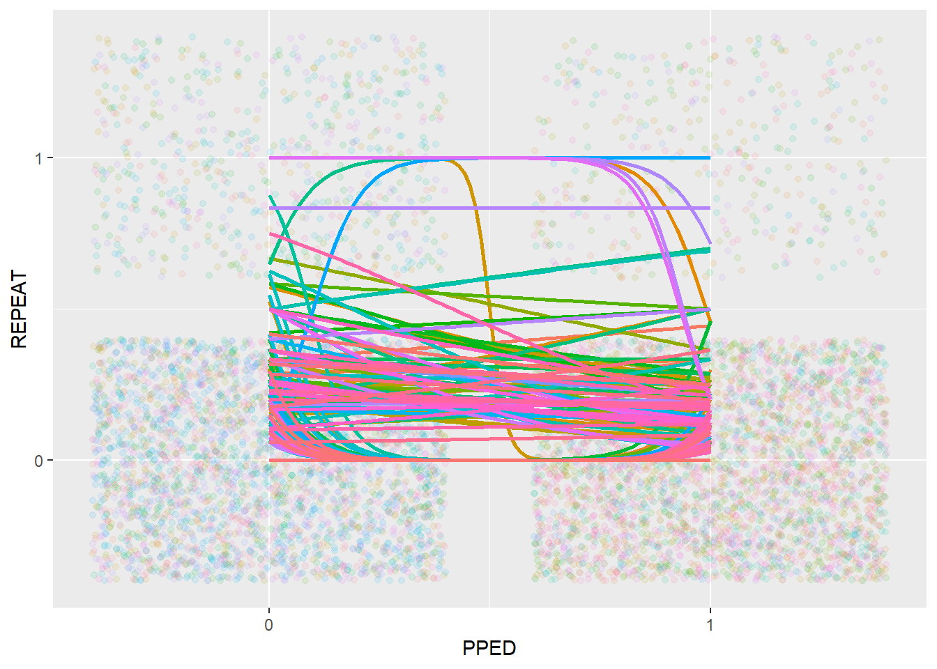
The relationship between PPED and REPEAT also appears to be quite different across schools. However, we can also see that most of the relationships follow a downward trend, going from 0 (no previous schooling) to 1 (with previous schooling), indicating a negative relationship between PPED and REPEAT.
Because of the observations above, we can conclude that there is a need for multilevel modelling in the current data, with not only a random intercept (SCHOOLID) but potentially also random slopes of the SEX and PPED.
7.1. Center Variables
Prior to fitting a multilevel model, it is necessary to center the predictors by using an appropriately chosen centering method (i.e. grand-mean centering or within-cluster centering), because the centering approach matters for the interpretation of the model estimates. Following the advice of Enders and Tofighi (2007), we should use within-cluster centering for the first-level predictors SEX and PPED, and grand-mean centering for the second-level predictor MSESC.
ThaiEdu_Center <- ThaiEdu_New %>%
  mutate(SEX = if_else(SEX == "girl", 0, 1),
         PPED = if_else(PPED == "yes", 1, 0)) %>%
  group_by(SCHOOLID) %>%
  mutate(SEX = SEX - mean(SEX),
         PPED = PPED - mean(PPED)) %>%
  ungroup() %>%
  mutate(MSESC = MSESC - mean(MSESC, na.rm = T))

head(ThaiEdu_Center)
## # A tibble: 6 x 5
## SCHOOLID SEX PPED REPEAT MSESC
## <fct> <dbl> <dbl> <dbl+lbl> <dbl>
## 1 10103 -0.647 -0.882 0 [no] 0.870
## 2 10103 -0.647 -0.882 0 [no] 0.870
## 3 10103 -0.647 0.118 0 [no] 0.870
## 4 10103 -0.647 0.118 0 [no] 0.870
## 5 10103 -0.647 0.118 0 [no] 0.870
## 6 10103 -0.647 0.118 0 [no] 0.8707.2. Intercept Only Model
To specify a multilevel model, we use the glmer function from the lme4 package. Note that the random effect term should be included in parentheses. In addition, within the parentheses, the random slope term(s) and the cluster terms should be separated by |. Note that we use an additional argument control = glmerControl(optimizer = "bobyqa", optCtrl = list(maxfun=2e5)) in the glmer function to specify a higher number of maximum iterations than default (10000). This might be necessary because a multilevel model may require a large number of iterations to converge.
We start by specifying an intercept-only model, in order to assess the impact of the clustering structure of the data.
Model_Multi_Intercept <- glmer(formula = REPEAT ~ 1 + (1|SCHOOLID),
                               family = binomial(logit),
                               data = ThaiEdu_Center,
                               control = glmerControl(optimizer = "bobyqa", optCtrl = list(maxfun=2e5)))

summary(Model_Multi_Intercept)
## Generalized linear mixed model fit by maximum likelihood (Laplace
## Approximation) [glmerMod]
## Family: binomial ( logit )
## Formula: REPEAT ~ 1 + (1 | SCHOOLID)
## Data: ThaiEdu_Center
## Control:
## glmerControl(optimizer = "bobyqa", optCtrl = list(maxfun = 2e+05))
##
## AIC BIC logLik deviance df.resid
## 5547.1 5560.9 -2771.5 5543.1 7514
##
## Scaled residuals:
## Min 1Q Median 3Q Max
## -1.6254 -0.4174 -0.2487 -0.1765 4.7824
##
## Random effects:
## Groups Name Variance Std.Dev.
## SCHOOLID (Intercept) 1.646 1.283
## Number of obs: 7516, groups: SCHOOLID, 356
##
## Fixed effects:
## Estimate Std. Error z value Pr(>|z|)
## (Intercept) -2.22480 0.08391 -26.51 <2e-16 ***
## ---
## Signif. codes: 0 '***' 0.001 '**' 0.01 '*' 0.05 '.' 0.1 ' ' 1Below we calculate the ICC (intra-class correlation) of the intercept-only model.
icc(Model_Multi_Intercept)##
## Intraclass Correlation Coefficient for Generalized linear mixed model
##
## Family : binomial (logit)
## Formula: REPEAT ~ 1 + (1 | SCHOOLID)
##
## ICC (SCHOOLID): 0.3334An ICC of 0.33 means that 33% of the variation in the outcome variable can be accounted for by the clustering stucture of the data. This provides evidence that a multilevel model may make a difference to the model estimates, in comparison with a non-multilevel model. Therefore, the use of multilevel models is necessary and warrantied.
7.3. Full Model
It is good practice to build a multilevel model step by step. However, as this tutorial’s focus is not on muitilevel modelling, we go directly from the intercept-only model to the full-model that we are ultimately interested in. In the full model, we include not only fixed effect terms of SEX, PPED and MSESC and a random intercept term, but also random slope terms for SEX and PPED. Note that we specify family = binomial(link = "logit"), as this model is essentially a binary logistic regression model.
Model_Multi_Full <- glmer(REPEAT ~ SEX + PPED + MSESC + (1 + SEX + PPED|SCHOOLID),
                          family = binomial(logit),
                          data = ThaiEdu_Center,
                          control = glmerControl(optimizer = "bobyqa", optCtrl = list(maxfun=2e5)))
## boundary (singular) fit: see ?isSingularsummary(Model_Multi_Full)## Generalized linear mixed model fit by maximum likelihood (Laplace
## Approximation) [glmerMod]
## Family: binomial ( logit )
## Formula: REPEAT ~ SEX + PPED + MSESC + (1 + SEX + PPED | SCHOOLID)
## Data: ThaiEdu_Center
## Control:
## glmerControl(optimizer = "bobyqa", optCtrl = list(maxfun = 2e+05))
##
## AIC BIC logLik deviance df.resid
## 5468.0 5537.2 -2724.0 5448.0 7506
##
## Scaled residuals:
## Min 1Q Median 3Q Max
## -2.4509 -0.4003 -0.2451 -0.1732 5.6938
##
## Random effects:
## Groups Name Variance Std.Dev. Corr
## SCHOOLID (Intercept) 1.66584 1.2907
## SEX 0.15439 0.3929 0.56
## PPED 0.04748 0.2179 -0.61 0.32
## Number of obs: 7516, groups: SCHOOLID, 356
##
## Fixed effects:
## Estimate Std. Error z value Pr(>|z|)
## (Intercept) -2.2727 0.0886 -25.652 < 2e-16 ***
## SEX 0.4093 0.1105 3.704 0.000212 ***
## PPED -0.5555 0.1534 -3.622 0.000292 ***
## MSESC -0.5054 0.2172 -2.327 0.019988 *
## ---
## Signif. codes: 0 '***' 0.001 '**' 0.01 '*' 0.05 '.' 0.1 ' ' 1
##
## Correlation of Fixed Effects:
## (Intr) SEX PPED
## SEX 0.017
## PPED 0.024 0.064
## MSESC 0.048 0.064 0.077
## convergence code: 0
## boundary (singular) fit: see ?isSingularThe results (pertaining to the fixed effects) are similar to the results of the previous binary logistic regression and binomial logistic regression models. On the pupil-level, SEX has a significant and positive influence on the odds of a pupil repeating a grade, while PPED has a significant and negative influence. On the school-level, MSESC has a significant and negative effect on the outcome variable. Let’s also look at the variance of the random effect terms.
Again, we can use the summ() function to retrieve the exponentiated coefficient estimates for easier interpretation.
summ(Model_Multi_Full, exp = T)## MODEL INFO:
## Observations: 7516
## Dependent Variable: REPEAT
## Type: Mixed effects generalized linear regression
## Error Distribution: binomial
## Link function: logit
##
## MODEL FIT:
## AIC = 5467.99, BIC = 5537.23
## Pseudo-R² (fixed effects) = 0.02
## Pseudo-R² (total) = 0.36
##
## FIXED EFFECTS:
##
## | | exp(Est.)| S.E.| z val.| p|
## |:-----------|---------:|----:|------:|----:|
## |(Intercept) | 0.10| 0.09| -25.65| 0.00|
## |SEX | 1.51| 0.11| 3.70| 0.00|
## |PPED | 0.57| 0.15| -3.62| 0.00|
## |MSESC | 0.60| 0.22| -2.33| 0.02|
##
## RANDOM EFFECTS:
##
## | Group | Parameter | Std. Dev. |
## |:--------:|:-----------:|:---------:|
## | SCHOOLID | (Intercept) | 1.29 |
## | SCHOOLID | SEX | 0.39 |
## | SCHOOLID | PPED | 0.22 |
##
## Grouping variables:
##
## | Group | # groups | ICC |
## |:--------:|:--------:|:----:|
## | SCHOOLID | 356 | 0.34 |We can also use the allEffects function to visualise the effects of the parameter estimates. Note that because the first-level categorical variables (SEX and PPED) are centered, they are treated as continuous variables in the model and as well in the following effect plots.
plot(allEffects(Model_Multi_Full))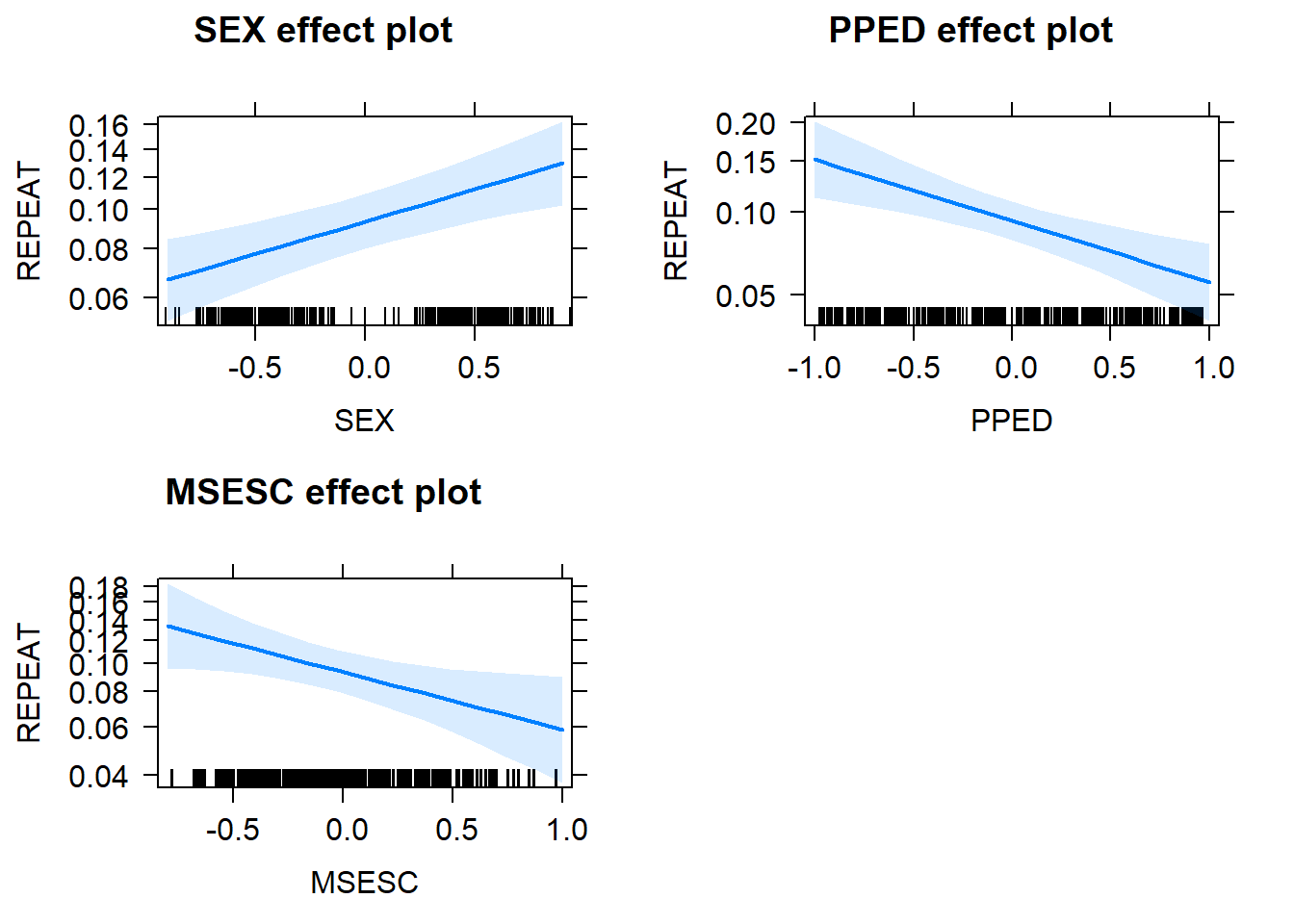
In addition to the fixed-effect terms, let’s also look at the random effect terms. From the ICC value before, we know that it’s necessary to include a random intercept. However, the necessity of including random slopes for SEX and PPED is less clear. To find this out, we can use the likelihood ratio test and AIC to judge whether the inclusion of the random slope(s) improves model fit.
#let's fit a less-than-full model that leaves out the random slope term of `SEX`
Model_Multi_Full_No_SEX <- glmer(REPEAT ~ SEX + PPED + MSESC + (1 + PPED|SCHOOLID),
                                 family = binomial(logit),
                                 data = ThaiEdu_Center,
                                 control = glmerControl(optimizer = "bobyqa", optCtrl = list(maxfun=2e5)))
## boundary (singular) fit: see ?isSingular#let's fit a less-than-full model that leaves out the random slope term of `PPED`
Model_Multi_Full_No_PPED <- glmer(REPEAT ~ SEX + PPED + MSESC + (1 + SEX|SCHOOLID),
family = binomial(logit),
data = ThaiEdu_Center,
control = glmerControl(optimizer = "bobyqa", optCtrl = list(maxfun=2e5)))
#let's fit a less-than-full model that leaves out the random slope terms of both `SEX` and `PPED`
Model_Multi_Full_No_Random_Slope <- glmer(REPEAT ~ SEX + PPED + MSESC + (1|SCHOOLID),
family = binomial(logit),
data = ThaiEdu_Center,
control = glmerControl(optimizer = "bobyqa", optCtrl = list(maxfun=2e5)))Likelihood ratio test:
#compare the full model with that model that excludes `SEX`
anova(Model_Multi_Full_No_SEX, Model_Multi_Full, test="Chisq")
## Data: ThaiEdu_Center
## Models:
## Model_Multi_Full_No_SEX: REPEAT ~ SEX + PPED + MSESC + (1 + PPED | SCHOOLID)
## Model_Multi_Full: REPEAT ~ SEX + PPED + MSESC + (1 + SEX + PPED | SCHOOLID)
## Df AIC BIC logLik deviance Chisq Chi Df
## Model_Multi_Full_No_SEX 7 5466.6 5515.1 -2726.3 5452.6
## Model_Multi_Full 10 5468.0 5537.2 -2724.0 5448.0 4.6054 3
## Pr(>Chisq)
## Model_Multi_Full_No_SEX
## Model_Multi_Full 0.2031#compare the full model with that model that excludes `PPED`
anova(Model_Multi_Full_No_PPED, Model_Multi_Full, test="Chisq")## Data: ThaiEdu_Center
## Models:
## Model_Multi_Full_No_PPED: REPEAT ~ SEX + PPED + MSESC + (1 + SEX | SCHOOLID)
## Model_Multi_Full: REPEAT ~ SEX + PPED + MSESC + (1 + SEX + PPED | SCHOOLID)
## Df AIC BIC logLik deviance Chisq Chi Df
## Model_Multi_Full_No_PPED 7 5462.9 5511.4 -2724.4 5448.9
## Model_Multi_Full 10 5468.0 5537.2 -2724.0 5448.0 0.9052 3
## Pr(>Chisq)
## Model_Multi_Full_No_PPED
## Model_Multi_Full 0.8242anova(Model_Multi_Full_No_Random_Slope, Model_Multi_Full, test="Chisq")## Data: ThaiEdu_Center
## Models:
## Model_Multi_Full_No_Random_Slope: REPEAT ~ SEX + PPED + MSESC + (1 | SCHOOLID)
## Model_Multi_Full: REPEAT ~ SEX + PPED + MSESC + (1 + SEX + PPED | SCHOOLID)
## Df AIC BIC logLik deviance Chisq
## Model_Multi_Full_No_Random_Slope 5 5463.2 5497.8 -2726.6 5453.2
## Model_Multi_Full 10 5468.0 5537.2 -2724.0 5448.0 5.2249
## Chi Df Pr(>Chisq)
## Model_Multi_Full_No_Random_Slope
## Model_Multi_Full 5 0.3891From the all insignificant likelihood ratio test results (Pr(>Chisq) > 0.05), we can conclude that there is no significant improvement in model fit by adding any random slope terms.
AIC:
AIC(logLik(Model_Multi_Full)) #full model## [1] 5467.985AIC(logLik(Model_Multi_Full_No_SEX)) #model without SEX## [1] 5466.591AIC(logLik(Model_Multi_Full_No_PPED)) #model without PPED## [1] 5462.89AIC(logLik(Model_Multi_Full_No_Random_Slope)) #model without random slopes## [1] 5463.21From the AIC results, we see that including random slope terms either does not substantially improve AIC (indicated by lower AIC value) or leads to worse AIC (i.e. higher). Therefore, we also conclude there is no need to include the random effect term(s).
8. Other Family (Distribution) and Link Functions
So far, we have introduced binary and binomial logistic regression, both of which come from the binomial family with the logit link. However, there are many more distribution families and link functions that we can use in glm analysis. For instance, to model binary outcomes, we can also use the probit link or the complementary log-log (cloglog) instead of the logit link. To model count data, we can also use Poisson regression, which assumes that the outcome variable comes from a Poisson distribution and uses the logarithm as the link function. For an overview of possible glm models, see the Wikipedia page for GLM.
References
Bates, D., Maechler, M., Bolker, B., & Walker, S. (2015). Fitting Linear Mixed-Effects Models Using lme4. Journal of Statistical Software, 67(1), 1-48. doi:10.18637/jss.v067.i01
Enders, C. K., & Tofighi, D. (2007). Centering predictor variables in cross-sectional multilevel models: A new look at an old issue. Psychological Methods, 12(2), 121-138. doi:10.1037/1082-989X.12.2.121
Fox, J. (2003). Effect Displays in R for Generalised Linear Models. Journal of Statistical Software, 8(15), 1-27. http://www.jstatsoft.org/v08/i15/
Long, JA. (2019). jtools: Analysis and Presentation of Social Scientific Data. R package version 2.0.1, https://cran.r-project.org/package=jtools
Lüdecke, D. (2019). sjstats: Statistical Functions for Regression Models (Version 0.17.5). doi: 10.5281/zenodo.1284472
Raudenbush, S. W., & Bhumirat, C. (1992). The distribution of resources for primary education and its consequences for educational achievement in Thailand. International Journal of Educational Research, 17(2), 143-164. doi:10.1016/0883-0355(92)90005-Q
Sing, T., Sander, O., Beerenwinkel, N. & Lengauer, T. (2005). ROCR: visualizing classifier performance in R. Bioinformatics, 21(20), pp. 7881. http://rocr.bioinf.mpi-sb.mpg.de
Wickham, H. (2017). tidyverse: Easily Install and Load the ‘Tidyverse’. R package version 1.2.1. https://CRAN.R-project.org/package=tidyverse