WAMBS-Checklist in SPSS
By Naomi Schalken, Lion Behrens, Laurent Smeets and Rens van de Schoot
Last modified: date: 03 november 2018
In this exercise you will be following the steps of the When-to-Worry-and-How-to-Avoid-the-Misuse-of-Bayesian-Statistics – checklist (the WAMBS-checklist) to analyze data of PhD-students.
We are continuously improving the tutorials so let me know if you discover mistakes, or if you have additional resources I can refer to. The source code is available via Github. If you want to be the first to be informed about updates, follow me on Twitter.
Example Data
The data we will be using for this exercise is based on a study about predicting PhD-delays ( Van de Schoot, Yerkes, Mouw and Sonneveld 2013). The data can be downloaded here. Among many other questions, the researchers asked the Ph.D. recipients how long it took them to finish their Ph.D. thesis (n=333). It appeared that Ph.D. recipients took an average of 59.8 months (five years and four months) to complete their Ph.D. trajectory. The variable B3_difference_extra measures the difference between planned and actual project time in months (mean=9.96, minimum=-31, maximum=91, sd=14.43).
For the current exercise we are interested in the question whether age of the Ph.D. recipients is related to a delay in their project.
Question: Write down the null and alternative hypothesis that represent this question. Which hypothesis do you deem more likely?
H0: Age is not related to the PhD project delays.
H1: Age is related to the PhD project delays.
The relation between completion time and age is expected to be non-linear. This might be due to that at a certain point in your life (i.e., midthirties), family life takes up more of your time than when you are in your twenties or when you are older.
So, in our model the GAP is the dependent variable and AGE and AGE2 are the predictors. The data can be found in the file phd-delays.csv .
Preparation – Importing and Exploring Data
You can find the data in the file phd-delays.csv, which contains all variables that you need for this analysis. Although it is a.csv-file, you can directly load it into SPSS using the following syntax:
/GET DATA  /TYPE=TXT
  /FILE="C: your working directory\phd-delays.csv"
  /ENCODING='UTF8'
  /DELCASE=LINE
  /DELIMITERS=";"
  /ARRANGEMENT=DELIMITED
  /FIRSTCASE=2
  /IMPORTCASE=ALL
  /VARIABLES=
  B3_difference_extra F2.0
  E4_having_child F1.0
  E21_sex F1.0
  E22_Age F2.0
  E22_Age_Squared F2.0.
CACHE.
EXECUTE.
Once you loaded in your data, it is advisable to check whether your data import worked well. Therefore, first have a look at the summary statistics of your data. You can do so by clicking Analyze -> Descriptive Statistics -> Descriptives . Also, the scatter plot of AGE and GAP can be checked, by Graphs -> Legacy Dialogs -> Scatter/Dot . Alternatively, to construct a reproducible analysis, you can open a new syntax file by clicking File -> New -> Syntax and executing the following syntax:
DESCRIPTIVES VARIABLES=B3_difference_extra E22_Age E22_Age_Squared
  /STATISTICS=MEAN STDDEV VARIANCE MIN MAX SEMEAN.

GRAPH
  /SCATTERPLOT(BIVAR)=E22_Age WITH B3_difference_extra
  /MISSING=LISTWISE.
Question: Have all your data been loaded in correctly? That is, do all data points substantively make sense? If you are unsure, go back to the .csv-file to inspect the raw data.
B3_difference_extra: Mean = 9.97, SE = 0.791
E22_Age: Mean = 31.68, SE = 0.376
E22_Age_Squared: Mean= 1050.22, SE=35.970
Step 1: Do you understand the priors?
Before actually looking at the data we first need to think about the prior distributions and hyperparameters for our model. For the current model, there are four priors:
- the intercept
- the two regression parameters (\(\beta_1\) for the relation with AGE and \(\beta_2\) for the relation with AGE2)
- the residual variance (\(\in\))
We first need to determine which distribution to use for the priors. Let’s use for the
- intercept a normal prior with \(\mathcal{N}(\mu_0, \sigma^{2}_{0})\), where \(\mu_0\) is the prior mean of the distribution and \(\sigma^{2}_{0}\) is the variance parameter
- \(\beta_1\) a normal prior with \(\mathcal{N}(\mu_1, \sigma^{2}_{1})\)
- \(\beta_2\) a normal prior with \(\mathcal{N}(\mu_2, \sigma^{2}_{2})\)
- \(\in\) an Inverse Gamma distribution with \(IG(\kappa_0,\theta_0)\), where \(\kappa_0\) is the shape parameter of the distribution and \(\theta_0\) the rate parameter
Next, we need to specify actual values for the hyperparameters of the prior distributions. Let’s say we found a previous study and based on this study the following hyperparameters can be specified:
- intercept\(\sim \mathcal{N}(10, 5)\)
- \(\beta_1 \sim \mathcal{N}(.8, 5)\)
- \(\beta_2 \sim \mathcal{N}(0, 10)\)
- \(\in \sim IG(0.001, 0.001)\)
Note: It is not possible to specify the prior variance for the intercept via the SPSS menu. However, it is possible to change in the syntax.
Run the model by pasting the following code in the syntax:
BAYES REGRESSION B3_difference_extra WITH E22_Age E22_Age_Squared
  /CRITERIA CILEVEL=95 TOL=0.000001 MAXITER=2000
  /DESIGN COVARIATES=E22_Age E22_Age_Squared
  /INFERENCE ANALYSIS=BOTH
  /PRIOR TYPE=CONJUGATE SHAPEPARAM=0.001 SCALEPARAM=0.001 MEANVECTOR=10 0.8 0 VMATRIX=5;0 5;0 0 10
  /ESTBF COMPUTATION=JZS COMPARE=NULL
  /PLOT COVARIATES=E22_Age_Squared E22_Age  INTERCEPT=TRUE ERRORVAR=TRUE BAYESPRED=TRUE.
Look at the prior distribution plots of all parameters. Resist looking at any other results for the moment.
Step 2: Run the model and check for convergence
Not possible yet to check for convergence in SPSS by using trace plots.
Question: What is the maximum number of iterations used in SPSS? Are you satisfied with the number of iterations used by the software?
The maximum number of iterations that is used by default = 2000.This number can be found in the syntax.
Not possible yet to check for convergence by means of the Gelman and Rubin diagnostic.
Question: What happens if the maximum number of iterations was much lower, such as 200?
_Then SPSS gives a warning message:_
| Warnings |
|---|
| During numerical integration, the maximum number of iterations was reached but convergence was not achieved. The value returned is the estimate of integral after the last iteration. You might try increasing the number of iterations. |
Step 3: doubling the number of iterations and convergence diagnostics
We want to be absolutely sure the model reached convergence and therefore you have to re-run the model with more than twice the number of iterations and compute the relative bias.
Fill out the table below using the formula to compute the relative bias for each parameter separately. So in the formula you need the parameter estimates of the initial converged analysis and the parameter estimates of the analysis with double iterations:
\[ \text{bias} \% = 100 \cdot \frac{\text{analysis with double iterations- initial converged analysis}}{\text{initial converged analysis}} \]
You should combine the relative bias in combination with substantive knowledge about the metric of the parameter of interest to determine when levels of relative deviation are negligible or problematic. For example, with a regression coefficient of 0.001, a 10% relative deviation level might not be substantively relevant. However, with an intercept parameter of 50, a 10% relative deviation level might be quite meaningful. The specific level of relative deviation should be interpreted in the substantive context of the model. Some examples of interpretations are:
- if relative deviation is < |5|%, then do not worry;
- if relative deviation > |5|%, then rerun with 4x nr of iterations.
| Parameters | Estimate model with max. iterations 2000 | Estimate model with max. iterations 4000 | Bias |
|---|---|---|---|
| Intercept | |||
| Age | |||
| Age2 | |||
| Residual variance |
Question: Are you satisfied with number of iterations, or do you want to re-run the model with even more iterations? Check the description in the WAMBS-checklist. Continue until you are satisfied.
| Parameters | Estimate model with max. iterations 2000 | Estimate model with max. iterations 4000 | Bias |
|---|---|---|---|
| Intercept | -39.414 | -39.414 | 0 |
| Age | 2.295 | 2.295 | 0 |
| Age2 | -0.022 | -0.022 | 0 |
| Residual variance | 197.522 | 197.522 | 0 |
You probably found no differences between the two analyses with a different number of maximum iterations. This is caused by the fact that SPSS stops running the analysis if convergence is reached. So the maximum number of iterations is not similar to the real number of iterations used. Fortunately, SPSS does give you a warning if convergence IS NOT reached, by providing a warning message. If such a situation occurs, you can decide to increase the number of maximum iterations, since this might lead to convergence.
Step 4: Does the posterior distribution histogram have enough precision?
Not yet available in SPSS to check posterior distribution histograms.
Step 5: Do the chains exhibit a strong degree of autocorrelation
Not yet available in SPSS to check autocorrelation plots.
Step 6: Does the posterior distribution make substantive sense?
The Kernel density plots are automatically given in the SPSS output for the parameters in the final model of
Question: What is your conclusion; do the posterior distributions make sense?
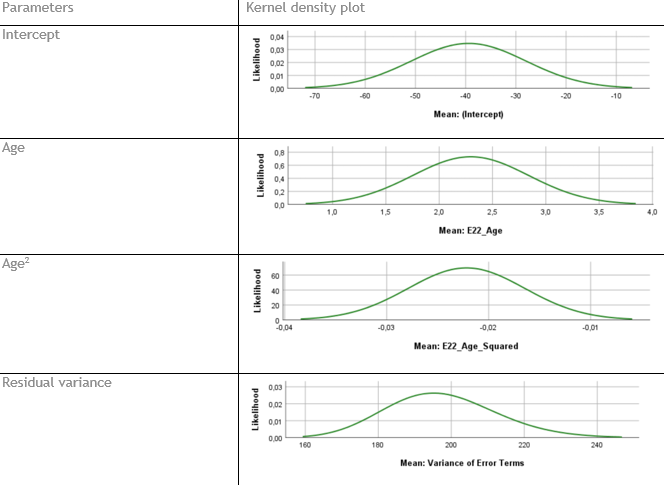
The plots show that the posterior distributions make sense.
Step 7: Do different specifications of the multivariate variance priors influence the results?
To understand how the prior on the residual variance impacts the posterior results, we compare the previous model with a model where different hyperparameters for the Inverse Gamma distribution are specified. The default prior in SPSS for the variance is a reference prior, which looks as follows:
Question: Are the results robust for different specifications of the prior on the residual variance?
| Parameters | Estimate with IG(.001, .001) | Estimate with IG (.5, .5) | Bias |
|---|---|---|---|
| Intercept | |||
| Age | |||
| Age2 | |||
| Residual variance |
| Parameters | Estimate with IG(.001, .001) | Estimate with IG (.5, .5) | Bias |
|---|---|---|---|
| Intercept | -39.414 | -39.414 | 0 |
| Age | 2.295 | 2.295 | 0 |
| Age2 | -0.022 | -0.022 | 0 |
| Residual variance | 197.522 | 196.931 | \(100\cdot \frac{196.931-197.522}{197.522} = 0.299\%\) |
Yes, the results are robust, because there is only a really small amount of relative bias for the residual variance.
Step 8: Is there a notable effect of the prior when compared with non-informative priors?
To understand the influence of the informative priors on the intercept and both regression coefficients, remove the prior specification in the input file. This way, the software will use its default prior settings.
Did this non-informative model reach convergence (think about all the previous steps)?
If so, compare the posterior parameters with the informative model and calculate the bias.
Question: What is your conclusion about the influence of the priors on the posterior results?
| Parameters | Estimates with default priors | Estimate with informative priors | Bias |
|---|---|---|---|
| Intercept | |||
| Age | |||
| Age2 | |||
| Residual variance |
| Parameters | Estimates with default priors SPSS | Estimate with informative priors | Bias |
|---|---|---|---|
| Intercept | -47.088 | -39.414 | \(100\cdot \frac{-39.414–47.088 }{-47.088} = 16.297 \%\) |
| Age | 2.657 | 2.295 | \(100\cdot \frac{2.295-2.657-}{2.657} = 13.624\%\) |
| Age2 | -0.026 | -0.022 | \(100 \cdot \frac{-0.022–0.026}{-0.026} = 15.385\%\) |
| Residual variance | 197.608 | 197.522 | \(100\cdot \frac{197.522-197.608}{197.608} = 0.044\%\) |
The informative priors have quite some influence on the posterior results.
Question: Which results will you use to draw conclusion on?
This really depends on where the priors come from. If for example your informative priors come from a reliable source, you should use them. The most important thing is that you choose your priors accurately, and have good arguments to use them. If not, you shouldn’t use really informative priors and use the results based on the non-informative priors.
Step 9: Are the results stable from a sensitivity analysis??
From the original WAMBS-paper:
“If informative or weakly-informative priors are used, then we suggest running a sensitivity analysis of these priors. When subjective priors are in place, then there might be a discrepancy between results using different subjective prior settings. A sensitivity analysis for priors would entail adjusting the entire prior distribution (i.e., using a completely different prior distribution than before) or adjusting hyperparameters upward and downward and re-estimating the model with these varied priors. Several different hyperparameter specifications can be made in a sensitivity analysis, and results obtained will point toward the impact of small fluctuations in hyperparameter values. [.] The purpose of this sensitivity analysis is to assess how much of an impact the location of the mean hyperparameter for the prior has on the posterior. [.] Upon receiving results from the sensitivity analysis, assess the impact that fluctuations in the hyperparameter values have on the substantive conclusions. Results may be stable across the sensitivity analysis, or they may be highly instable based on substantive conclusions. Whatever the finding, this information is important to report in the results and discussion sections of a paper. We should also reiterate here that original priors should not be modified, despite the results obtained.”
If you still have time left, you can adjust the hyperparameters for the priors upward and downward and re-estimate the model with these different priors to check for robustness.
Question : What is your conclusion about the sensitivity analyses?
Step 10: Is the Bayesian way of interpreting and reporting model results used?
After Points 1-9 have been carefully considered and addressed, model interpretation and the reporting of results become the next concern. For inspiration how to do this, check Appendix A of the WAMBS-paper or read the paper “Bayesian analyses: where to start and what to report”.
References
Depaoli, S., & Van de Schoot, R. (2017). Improving transparency and replication in Bayesian statistics: The WAMBS-Checklist. Psychological Methods, 22(2), 240.
Van de Schoot, R., & Depaoli, S. (2014). Bayesian analyses: Where to start and what to report. European Health Psychologist, 16(2), 75-84.