jamovi for Bayesian analyses with default priors
Ihnwhi Heo and Rens van de Schoot
Department of Methodology and Statistics, Utrecht University
Last modified: 02 November 2020
This tutorial explains how to conduct Bayesian analyses in jamovi (The jamovi project, 2020) with default priors for starters. With step-by-step illustrations, we perform and interpret core results of correlation analysis, multiple linear regression, t-test, and one-way analysis of variance, all from a Bayesian perspective. To enhance readers’ understanding, a brief comparison between the Bayesian and frequentist approach is provided in each analytic option. After the tutorial, we expect readers can perform basic Bayesian analyses and distinguish its approach from the frequentist approach.
If readers need fundamentals of jamovi and ways to interpret results from a frequentist statistics viewpoint, we recommend following jamovi for beginners. The current tutorial presumes that readers are familiar with conducting and interpreting frequentist statistical analyses in jamovi.
Since we continuously improve the tutorials, let us know if you discover mistakes, or if you have additional resources we can refer to. If you want to be the first to be informed about updates, follow Rens on Twitter.
How to cite this tutorial in APA style
Heo, I., & Van de Schoot, R. (2020, November). Tutorial: jamovi for Bayesian analyses with default priors. Zenodo. https://doi.org/10.5281/zenodo.4117882
Popularity Dataset
We will use a popularity dataset (Van de Schoot, 2020) from Van de Schoot, Van der Velden, Boom, and Brugman (2010). To download the dataset, click here.
The dataset is based on a study that investigates an association between popularity status and antisocial behavior from at-risk adolescents (n = 1,491), where gender and ethnic background are moderators under the association. The study distinguished subgroups within the popular status group in terms of overt and covert antisocial behavior.
For more information on the sample, instruments, methodology, and research context, we refer the interested readers to the paper (see references). A brief description of the variables in the dataset follows. The variable names in the table below will be used in the tutorial, henceforth.
| Variable name | Description |
|---|---|
| respnr | Respondents’ number |
| Dutch | Respondents’ ethnic background (0 = Dutch origin, 1 = non-Dutch origin) |
| gender | Respondents’ gender (0 = boys, 1 = girls) |
| sd | Adolescents’ socially desirable answering patterns |
| covert | Covert antisocial behavior |
| overt | Overt antisocial behavior |
How to cite the dataset in APA style
Van de Schoot, R. (2020). Popularity Dataset for Online Stats Training [Data set]. Zenodo. https://doi.org/10.5281/zenodo.3962123
I. Is a dataset on board?
- A dataset is a prerequisite for statistical analysis.
- To download the dataset that we will use (
popular_regr_1), click here. - With several mouse clicks, we can conveniently load the data. Do you remember two ways of loading data in jamovi? One is from your machine and the other is from the in-built data library.
- We expect you are familiar with loading the data.
- If not, please go to jamovi for beginners and see steps to load the data.
II. Another ‘earth’: Bayesian statistics
- Bayesian statistics and frequentist statistics are two different branches in the world of statistics. Their distinctive approaches lead to different ways of statistical inference. Therefore, they live on their respective earth.
- We provide ideas of Bayesian statistics briefly. Still, we refer interested readers to the two great easily-written papers for a more concrete explanation.
- A gentle introduction to Bayesian analysis: Applications to developmental research (Van de Schoot, Kaplan, Denissen, Asendorpf, Neyer, & Van Aken, 2014)
- Bayesian analyses: Where to start and what to report (Van de Schoot & Depaoli, 2014)
1. Bayesian parameter estimation
- In Bayesian statistics, the prior distributions are combined with the likelihood of data to update the prior distributions to the posterior distributions (see Van de Schoot et al., 2014 for introduction and application of Bayesian analysis). The updated posterior distributions about parameters of interest are used for statistical inference. This logic of Bayesian statistics implies that how the prior distributions are specified plays a crucial role in doing Bayesian statistics.
2. Bayesian hypothesis testing
- Bayesian hypothesis testing focuses on which hypothesis receives relatively more support from the observed data. This is quantified by the Bayes factor (Kass & Rafter, 1995).
- Say we are considering two hypotheses: the null hypothesis (\(H_{0}\)) and the alternative hypothesis (\(H_{1}\)). If the Bayes factor in favor of the alternative hypothesis (i.e., \(BF_{10}\)) is 15, this means that the support in the observed data is about fifteen times larger for the alternative hypothesis than for the null hypothesis. In this way, how likely the data are to be observed among competing hypotheses is expressed in terms of the Bayes factor.
- Please note that we do not use words such as significant and p-value in Bayesian statistics. They are the terms used under the frequentist framework.
3. Obtaining reproducible results in Bayesian statistics with a seed value
- Bayesian inference is based on the posterior distribution of parameters after taking into account the likelihood of data and the prior distribution. The likelihood and the prior are in the form of mathematical functions.
- The potential problem that could arise is that, usually, the posterior distribution is hard to get analytically (see Chapter 5 and Chapter 6 in Kruschke, 2014 for information about conjugate and non-conjugate prior). To solve this issue, Bayesian statistics uses the random number generator to approximate the posterior distribution. Due to generating random numbers, results from Bayesian analyses are slightly different each time we run Bayesian analyses.
- Surprisingly, this is not completely random such that each software has its hidden rule that the sequence of random numbers is generated! We can thus say the software is based on a pseudorandom number generator. The idea is that, whenever a certain number is fed as an input to the generator, the software produces the same sequence of pseudorandom numbers. Therefore, researchers and statisticians feed a specific number to the statistical software to make it reproduce the same outputs. For more information about setting seed values for Bayesian statistics, see Chapter 7 in Kruschke (2014).
- This tutorial is based on the jsq module version 1.0.1 where setting a seed value is not supported at the moment. Therefore, we kindly advise readers to be aware of this concern and not to be surprised if the Bayesian analyses with jamovi do not produce the same results each time.
III. Take-off to perform Bayesian analyses
- Please note that the jsq module should be installed on jamovi to perform Bayesian analyses. We assume that readers are prepared for the jsq module.
- If you are not familiar with downloading modules, please go to jamovi for beginners and see procedures to install modules.
- In each analysis, we provide a brief comparison between the frequentist and the Bayesian approach for the chosen analysis. The procedures to perform the Bayesian analysis follows the comparison. Next, you encounter the interpretation of results.
- For all the assumptions required for subsequent analyses, let’s assume that those assumptions are met.
1. Correlation analysis
- When you want to investigate the strength of the relationship between two variables, correlation analysis can be a choice.
- In frequentist statistics, the focus is to examine whether the correlation coefficient is significantly different from 0 or not. The significance level is usually set to .05. If a p-value is lower than the significance level, the null hypothesis that the correlation coefficient between two variables is 0 is rejected. The alternative hypothesis is that the correlation coefficient is not equal to 0.
- In Bayesian statistics, the null hypothesis postulates that the correlation coefficient between the two variables is 0. That is, the null hypothesis states that the two variables are not correlated. The alternative hypothesis, however, states that the correlation coefficient exists. In other words, two variables are correlated.
- Between the null and the alternative hypothesis, Bayesian statistics quantifies the relative support toward each hypothesis from observed data. The Bayes factor shows this quantification of support. In jamovi, the default Bayes factor is \(BF_{10}\). This value means how much the observed data relatively supports the alternative hypothesis (\(H_{1}\)) than the null hypothesis (\(H_{0}\)).
- For a better understanding, let’s test whether two variables in the dataset, the covert and overt antisocial behavior (covert and overt) are correlated.
- Go to the analyses ribbon -> Click Regression -> Bayesian Correlation Matrix under the Bayesian (jsq) header
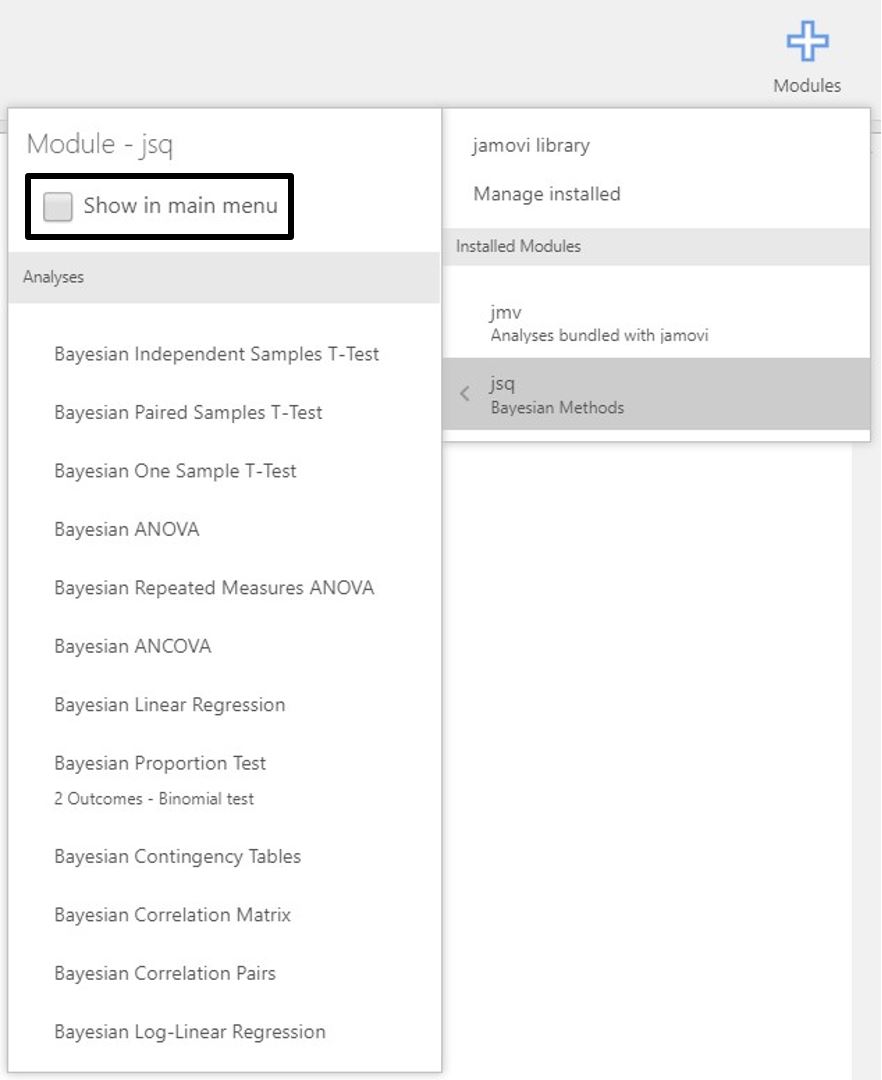
- If you cannot find the Bayesian analytic options although the jsq module is installed, this could be the possible solution. When you click the plus button and click the jsq module under the Installed Modules header, you can see whether ‘Show in main menu’ is checked or not.
- If ‘Show in main menu’ is unchecked like the picture below, you should check it to see Bayesian analytic options in the analyses ribbon!
- Move covert and overt to the right section. Next, check Credible intervals in the options panel.
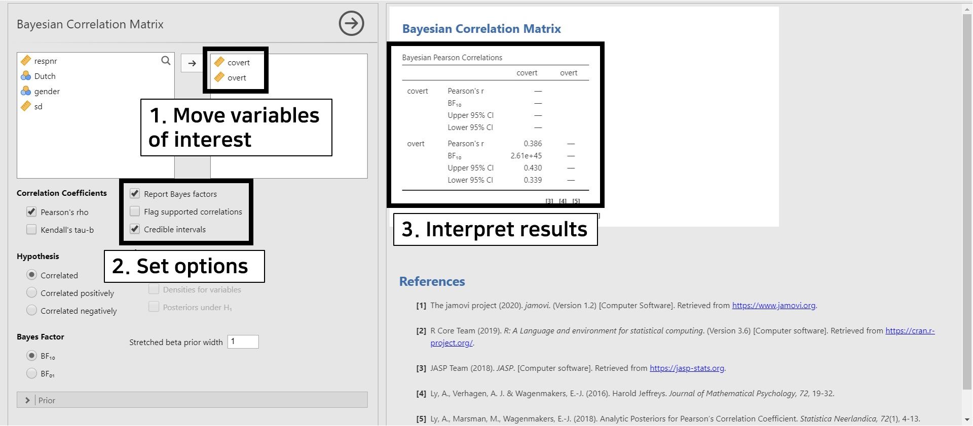
- The correlation coefficient between covert and overt is 0.386, and the \(BF_{10}\) is 2.61e+45. The number 2.61e+45 equals \(2.61 × 10^{45}\). We can interpret this result in a way that the support in the observed data is about \(2.61 × 10^{45}\) times larger for the alternative hypothesis (i.e., covert and overt are correlated) than for the null hypothesis (i.e., covert and overt are not correlated).
- The upper and lower limit of 95% credible interval are 0.430 and 0.339. Since 0 is not included in the 95% credible interval, there is a 95% probability that the correlation coefficient between covert and overt lies within the corresponding interval in the population. Therefore, it is fairly sure that covert and overt are correlated.
- Note that the Bayesian statistics is not concerned with rejecting or not rejecting the null hypothesis. Instead, it is keen on how much the observed data supports the alternative or the null hypothesis.
2. Multiple linear regression
- When you are interested in predicting outcomes of a continuous dependent variable with multiple continuous or categorical independent variables, multiple linear regression is performed.
- In the frequentist framework, we examine whether the regression coefficient is significantly different from 0. If the p-value is lower than the significance level, the null hypothesis that the regression coefficient is 0 is rejected. The alternative hypothesis is that the regression coefficient is not equal to 0.
- In the Bayesian framework, the null hypothesis states that the independent variables do not predict the dependent variables. The alternative hypothesis states that there exist effects of independent variables in predicting the dependent variables.
- For illustrative purposes, let’s predict adolescent’s socially desirable answering patterns (sd) with overt and covert antisocial behavior (overt and covert). Thus, we use sd as the dependent variable and covert and overt as the independent variables.
- Go to the analyses ribbon -> Click Regression -> Bayesian Linear Regression under the Bayesian (jsq) header
- Move sd to the Dependent Variable section and covert and overt to the Covariates section. Check Posterior summary under Output in the options panel. Note that the Best model is chosen by default. This means that we see the estimates under the most probable model after observing the data.
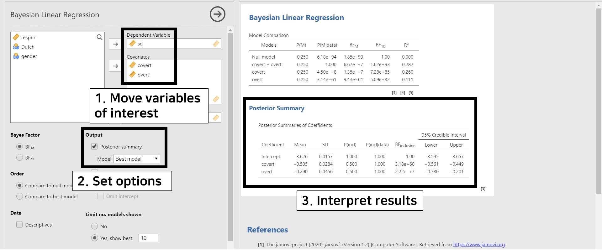
- To interpret the results, take a look at the table under Poster Summary in the results panel. As the title ‘Posterior Summary’ implies, statistical inferences in Bayesian statistics concentrate on the posterior distribution. The posterior summary shows the summary of regression coefficients after taking into account the default prior and the likelihood of data. The Mean and the SD refers to the posterior mean and the posterior standard deviation.
- The posterior mean of covert is -0.505. This is interpreted such that one unit increase in covert leads to a decrease of 0.505 unit in sd, on average. The 95% credible interval of [-0.561, -0.449] indicates that there is a 95% probability that the regression coefficient of covert lies within the corresponding credible interval in the population. Also, 0 is not included in the 95% credible interval, so there is fair evidence that covert predicts sd.
- The posterior mean of overt is -0.290. We can interpret this value in a way that, on average, one unit increase in overt leads to a decrease of 0.290 unit in sd. According to the 95% credible interval of [-0.380, -0.201], we are 95% sure that the regression coefficient of overt lies within the corresponding interval in the population. Moreover, the 95% credible interval does not include 0. Therefore, it is fairly sure that there is an effect of overt in predicting sd.
3. t-test
- A t-test can be used when you are interested in examining whether the means of certain variables between the two groups are different from each other.
- From a frequentist perspective, the focus is to examine whether the means between the two groups are significantly different. If the p-value is lower than the significance level, the null hypothesis that the mean difference between the two groups equals 0 is rejected. The alternative hypothesis states that the mean difference is significantly different from 0.
- From a Bayesian perspective, the null hypothesis states that there is no mean difference between the two groups. The alternative hypothesis, on the other hand, is that there is a mean difference between the two groups.
- As an instance, let’s investigate if the means of covert antisocial behavior (covert) between the respondents’ different ethnic backgrounds (Dutch) are different.
- Go to the analyses ribbon -> Click T-Tests -> Bayesian Independent Samples T-Test under the Bayesian (jsq) header
- Since we assumed that all assumptions are met, we use Student’s t-test. If the assumption of independent samples is violated, you can use Mann-Whitney U-test in the options panel.
- Move covert to the Dependent Variables section and Dutch to the Grouping Variable section.
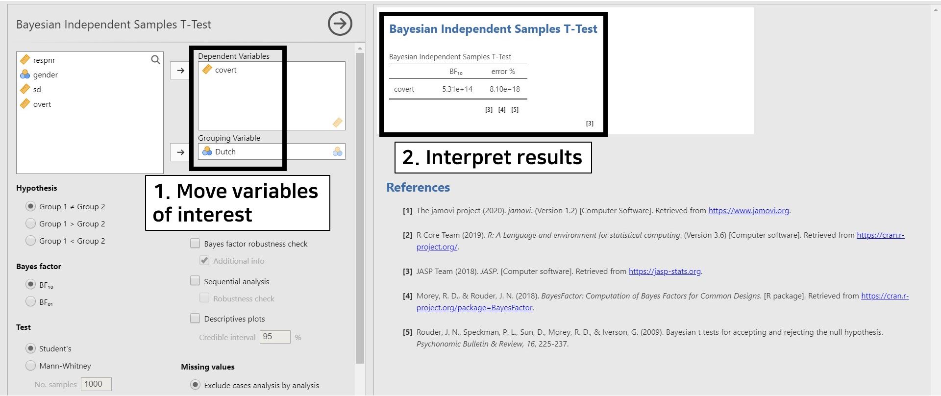
- Look at the table under the Bayesian Independent Samples T-Test. The number 5.31e+14 of \(BF_{10}\) equals \(5.31 × 10^{14}\). This result means that the observed data support \(5.31 × 10^{14}\) times more for the alternative hypothesis (i.e., there is a mean difference of covert between the two groups of the Dutch variable) than for the null hypothesis (i.e., A mean difference of covert between the two groups of the Dutch variable does not exist).
- The error % (error percentage) tells whether the numerical results are robust. According to the error % column, the error percentage is 8.10e-18, which is equal to \(8.10 × 10^{-18}\). Since the error percentage is low enough, we can say that the numerical results are robust.
4. One-way analysis of variance
- When you are keen on investigating if the means are different across groups, a one-way analysis of variance answers your question.
- In frequentist statistics, we aim to examine whether the means across different groups are significantly different from each other. If the p-value is lower than the significance level, the null hypothesis that there is no mean difference across groups is rejected. The alternative hypothesis states that there exist significant mean differences across groups.
- In Bayesian statistics, the null hypothesis states that there is no mean difference across different groups. The alternative hypothesis, on the other hand, says that there exist mean differences across different groups.
- For example, we will investigate whether the differences in the mean of covert antisocial behavior (covert) exist across respondents’ genders (gender).
- Before proceeding further, we should do one thing in advance. In the dataset, the gender variable has three categories, which are 0, 1, and 99. Because jamovi treats 99 as an independent category, which should not be the case, it is necessary to filter 99 out. We expect you are familiar with filtering.
- If not, please go to jamovi for beginners and see how to filter a certain category of the variable out.
- We proceed with the next procedure conditional on that you filtered the 99 category of the gender variable out!
- Go to the analyses ribbon -> Click ANOVA -> Bayesian ANOVA under the Bayesian (jsq) header
- Move covert to the Dependent Variable section and gender to the Fixed Factors section.
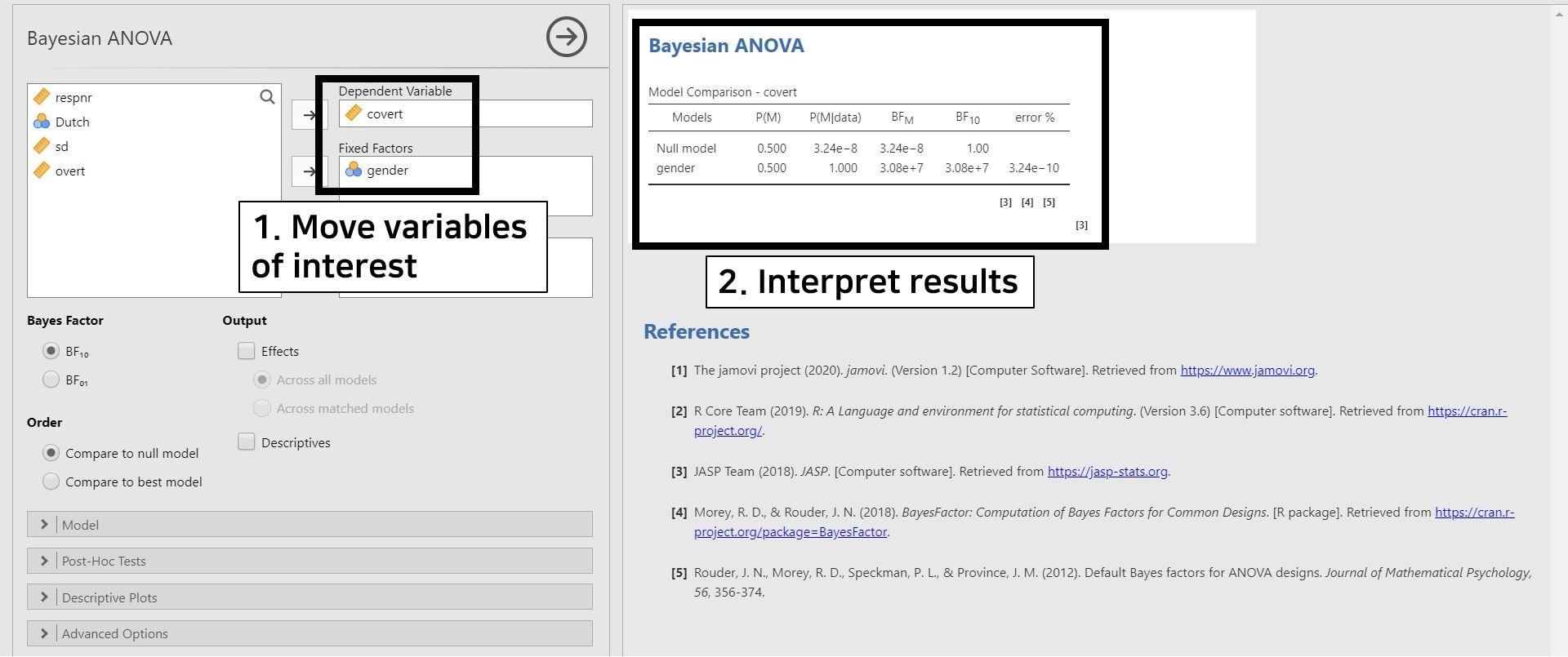
- Look at the table under the Bayesian ANOVA in the results panel. The Null model in the Models column only contains the grand mean. The gender model (denoted as gender in the Models column) adds an effect of the gender variable to the Null model. Consequently, we should look at the ‘gender’ model row.
- The value 3.08e+7 of \(BF_{10}\) is equal to \(3.08 × 10^{7}\). This value means that the support is \(3.08 × 10^{7}\) times larger for the alternative hypothesis (i.e., there exists mean differences of covert across gender groups) than for the null hypothesis (i.e., mean differences of covert do not exist across gender groups).
- As explained in the t-test part, error % indicates the robustness of results. The error percentage of 3.24e-10 equals \(3.24 × 10^{-10}\). This value is lower enough to show that the results are stable.
IV. Epilogue
- Congratulations! You have finished all the materials. We hope you found it informative.
- This tutorial covered simple but core steps excluding other advanced options. It should be noted, however, that there are more interesting concepts to illustrate in performing Bayesian statistical analysis.
- We thus recommend following the tutorial Advanced Bayesian regression in jamovi. It covers advanced options in conducting Bayesian regression analysis with a detailed explanation.
References
Kass, R. E., & Raftery, A. E. (1995). Bayes factors. Journal of the American Statistical Association, 90(430), 773-795.
Kruschke, J. (2014). Doing Bayesian Data Analysis: A Tutorial with R, JAGS, and Stan (2nd ed.). Academic Press.
The jamovi project. (2020). jamovi (Version 1.2.27)[Computer software].
Van de Schoot, R. (2020). Popularity Dataset for Online Stats Training [Data set]. Zenodo. https://doi.org/10.5281/zenodo.3962123
Van de Schoot, R., & Depaoli, S. (2014). Bayesian analyses: Where to start and what to report. The European Health Psychologist, 16(2), 75-84.
Van de Schoot, R., Kaplan, D., Denissen, J., Asendorpf, J. B., Neyer, F. J., & Van Aken, M. A. (2014). A gentle introduction to Bayesian analysis: Applications to developmental research. Child development, 85(3), 842-860. https://doi.org/10.1111/cdev.12169
Van de Schoot, R., Van der Velden, F., Boom, J., & Brugman, D. (2010). Can at-risk young adolescents be popular and anti-social? Sociometric status groups, anti-social behaviour, gender and ethnic background. Journal of adolescence, 33(5), 583-592. https://doi.org/10.1016/j.adolescence.2009.12.004