First Bayesian Inference: SPSS (regression analysis)
By Naomi Schalken, Lion Behrens, Laurent Smeets and Rens van de Schoot
Last modified: date: 03 november 2018
This tutorial provides the reader with a basic tutorial how to perform and interpret a Bayesian regression in SPSS. Throughout this tutorial, the reader will be guided through importing datafiles, exploring summary statistics and performing multiple regression. Here, we will exclusively focus on Bayesian statistics. In this tutorial, we start by using the default prior settings of the software. In a second step, we will apply user-specified priors, and if you really want to use Bayes for your own data, we recommend to follow the WAMBS-checklist, also available as SPSS-exercise.
We are continuously improving the tutorials so let me know if you discover mistakes, or if you have additional resources I can refer to. The source code is available via Github. If you want to be the first to be informed about updates, follow me on Twitter.
Preparation
This Tutorial Expects:
- Basic knowledge of hypothesis testing
- Basic knowledge of correlation and regression
- Basic knowledge of Bayesian inference
- Any installed version of SPSS higher than 25
Example Data
The data we will be using for this exercise is based on a study about predicting PhD-delays ( Van de Schoot, Yerkes, Mouw and Sonneveld 2013).The data can be downloaded here. Among many other questions, the researchers asked the Ph.D. recipients how long it took them to finish their Ph.D. thesis (n=333). It appeared that Ph.D. recipients took an average of 59.8 months (five years and four months) to complete their Ph.D. trajectory. The variable B3_difference_extra measures the difference between planned and actual project time in months (mean=9.96, minimum=-31, maximum=91, sd=14.43). For more information on the sample, instruments, methodology and research context we refer the interested reader to the paper.
For the current exercise we are interested in the question whether age of the Ph.D. recipients is related to a delay in their project.
The relation between completion time and age is expected to be non-linear. This might be due to the fact that at a certain point in your life priorities shift (i.e., in your mid thirties family life takes up more of your time than when you are younger or older).
So, in our model the GAP is the dependent variable and AGE and AGE2 are the predictors. The data can be found in the file phd-delays.csv.
Question: Write down the null and alternative hypothesis that represent this question.
H0: \(Age^2\) is not related to the PhD project delays.
H1: \(Age^2\) is related to the PhD project delays.
Preparation – Importing and Exploring Data
You can find the data in the file phd-delays.csv, which contains all variables that you need for this analysis. Although it is a .csv-file, you can directly load it into SPSS. If you do not know how, go to our How to Get Started With SPSS-exercise.
Once you loaded in your data, it is advisable to check whether your data import worked well. Therefore, first have a look at the summary statistics of your data (again, if you do not know how to obtain these estimates go to our How to Get Started With SPSS-exercise).
Regression – Default Priors
In this exercise you will investigate the impact of Ph.D. students’ \(age\) and \(age^2\) on the delay in their project time, which serves as the outcome variable using a regression analysis (note that we ignore assumption checking!).
As you know, Bayesian inference consists of combining a prior distribution with the likelihood obtained from the data. Specifying a prior distribution is one of the most crucial points in Bayesian inference and should be treated with your highest attention (for a quick refresher see e.g. Van de Schoot et al. 2017). In this tutorial, we will first rely on the default prior settings, thereby behaving a ‘naïve’ Bayesians (which might notalways be a good idea).
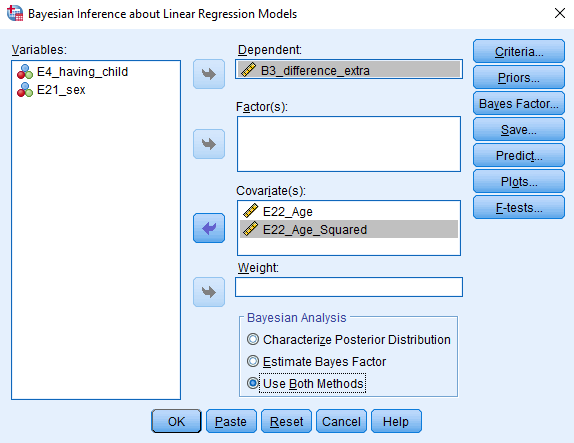
You can conduct the regression by clicking Analyze -> Bayesian Statistics -> Linear Regression. In the Bayes Factor tab, be sure to request both the posterior distribution and a Bayes factor by ticking Use Both Methods. Under Plots, be sure to request output for both covariates that you are using.
Alternatively, you can execute the following code in your syntax file:
BAYES REGRESSION B3_difference_extra WITH E22_Age E22_Age_Squared
  /CRITERIA CILEVEL=95 TOL=0.000001 MAXITER=2000
  /DESIGN COVARIATES=E22_Age E22_Age_Squared
  /INFERENCE ANALYSIS=BOTH
  /PRIOR TYPE=REFERENCE
  /ESTBF COMPUTATION=JZS COMPARE=NULL
  /PLOT COVARIATES=E22_Age_Squared E22_Age  INTERCEPT=FALSE ERRORVAR=FALSE BAYESPRED=FALSE.
The results that stem from a Bayesian analysis are genuinely different from those that are provided by a frequentist model. The key difference between Bayesian statistical inference and frequentist statistical methods concerns the nature of the unknown parameters that you are trying to estimate. In the frequentist framework, a parameter of interest is assumed to be unknown, but fixed. That is, it is assumed that in the population there is only one true population parameter, for example, one true mean or one true regression coefficient. In the Bayesian view of subjective probability, all unknown parameters are treated as uncertain and therefore are be described by a probability distribution. Every parameter is unknown, and everything unknown receives a distribution.
This is why in frequentist inference, you are primarily provided with a point estimate of the unknown but fixed population parameter. This is the parameter value that, given the data, is most likely in the population. An accompanying confidence interval tries to give you further insight in the uncertainty that is attached to this estimate. It is important to realize that a confidence interval simply constitutes a simulation quantity. Over an infinite number of samples taken from the population, the procedure to construct a (95%) confidence interval will let it contain the true population value 95% of the time. This does not provide you with any information how probable it is that the population parameter lies within the confidence interval boundaries that you observe in your very specific and sole sample that you are analyzing.
In Bayesian analyses, the key to your inference is the parameter of interest’s posterior distribution. It fulfills every property of a probability distribution and quantifies how probable it is for the population parameter to lie in certain regions. On the one hand, you can characterize the posterior by its mode. This is the parameter value that, given the data and its prior probability, is most probable in the population. Alternatively, you can use the posterior’s mean or median. Using the same distribution, you can construct a 95% credibility interval, the counterpart to the confidence interval in frequentist statistics. Other than the confidence interval, the Bayesian counterpart directly quantifies the probability that the population value lies within certain limits. There is a 95% probability that the parameter value of interest lies within the boundaries of the 95% credibility interval. Unlike the confidence interval, this is not merely a simulation quantity, but a concise and intuitive probability statement. For more on how to interpret Bayesian analysis, check Van de Schoot et al. 2014.
Question: Interpret the estimated effect, its interval and the posterior distribution.
\(Age\) seems to be a relevant predictor of PhD delays, with a posterior mean regression coefficient of 2.657, 95% Credibility Interval [1,504, 3.801]. Also, \(age^2\) seems to be a relevant predictor of PhD delays, with a posterior mean of -0.026, and a 95% Credibility Interval of [-0.038, -0.014]. The 95% Credibility Interval shows that there is a 95% probability that these regression coefficients in the population lie within the corresponding intervals, see also the posterior distributions in the figures below. Since 0 is not contained in the Credibility Interval we can be fairly sure there is an effect.

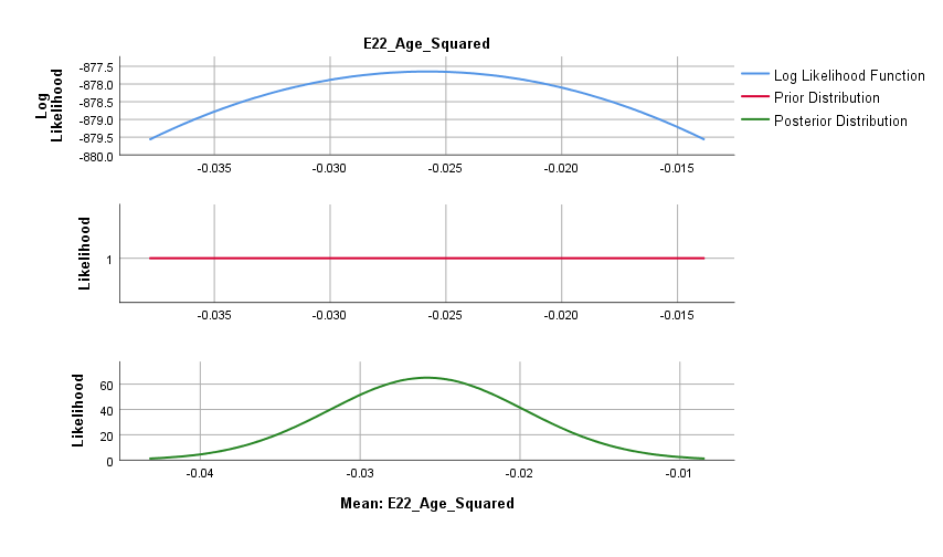
Question: Every Bayesian model uses a prior distribution. Describe the shape of the prior distribution.
The priors used are (almost) flat and allow probability mass across the entire parameter space. SPSS makes use of very wide normal distributions to come to this uninformative prior.
In statistical inference, there is a fundamental difference between estimating a population parameter and testing hypotheses regarding it. So far, you gave estimation-based interpretations by characterizing the parameter’s posterior distribution. Now, you are going to test hypotheses with the Bayes factor, the counterpart of the frequentist p-value. Other than the p-value that tries to reject a null hypothesis, the Bayes factor directly compares the evidence for two (or more) hypotheses under consideration. Above, you formulated the null and alternative hypothesis for the research question under investigation. A Bayes factor compares the likelihood of population parameter values under all scenarios that are in line with the null hypothesis with their likelihood under all scenarios that are in line with the alternative hypothesis. Ultimately, it quantifies how much better the alternative hypothesis fits better than the null and vice versa. It thus directly compares two hypotheses and provides evidence for both, something that the p-value cannot do.
Question: Interpret the Bayes Factor.
The Bayes factor = 123.528 for the current regression model. This means there is 123 time more support in the data for the model including the predictors when compared to an intercept only model.
Regression – User-specified Priors
In SPSS, you can also manually specify your prior distributions. Be aware that usually, this has to be done BEFORE peeking at the data, otherwise you are double-dipping (!). In theory, you can specify your prior knowledge using any kind of distribution you like. However, if your prior distribution does not follow the same parametric form as your likelihood, calculating the model can be computationally intense. Conjugate priors avoid this issue, as they take on a functional form that is suitable for the model that you are constructing. For your normal linear regression model, conjugacy is reached if the priors for your regression parameters are specified using normal distributions (und the residual variance receives an inverse gamma distribution, which is neglected here). In SPSS, you can only specify informative priors that are conjugate.
Let’s re-specify the regression model of the exercise above, using conjugate priors. For now we ignore the intercept prior specification, and set this to what we found in the analysis above, which is approximately \(N(-47, 153)\). We also leave the prior for the residual variance untouched for the moment. Regarding your regression parameters, you need to specify the hyperparameters of their normal distribution, which are the mean and the variance. The mean indicates which parameter value you deem most likely. The variance expresses how certain you are about that. We try 4 different prior specifications, for both the age coefficient, and the age squared coefficient. Since we cannot adapt the intercept prior via the analysis menu, we use the syntax to adapt the prior specifications.
To adapt the prior specifications SPSS works with a vector for the prior means (MEANVECTOR) and a covariance matrix for the variances. In this example we have 3 means (intercept and two regression coefficients) and thus a vector of length 3, in which values are separated by a space.
- So to get the prior mean vector of \(\begin{bmatrix}\beta_{intercept}\\& \beta_{age}\\& &\beta_{age^2}\end{bmatrix}\) use
MEANVECTOR= intercept age age2 - The covariance matrix is of the size 3×3, with the variances on the diagonal and 0 on all other places. These off-diagonal values are 0, because we do not expect a prior covariance between regression coefficients. Since the covariance matrix is symmetrical we only have to specify the bottom triangle. The different rows are separated by a “;”. So to get variance matrix \(\begin{bmatrix}variance_{intercept} & &\\0 & variance_{age} & \\0 & 0 & variance_{age^2}\end{bmatrix}\) use
VMATRIX= intercept; 0 age ;0 0 age2
First, we use the following prior specifications:
\(Age\) ~ N( 3, 0.4)
\(age^2\) ~ N( 0, 0.1)
Use the following syntax:
BAYES REGRESSION B3_difference_extra WITH E22_Age E22_Age_Squared
  /CRITERIA CILEVEL=95 TOL=0.000001 MAXITER=2000
  /DESIGN COVARIATES=E22_Age E22_Age_Squared
  /INFERENCE ANALYSIS=BOTH
  /PRIOR TYPE=CONJUGATE SHAPEPARAM=2 SCALEPARAM=2 MEANVECTOR=-47 3 0 VMATRIX= 153; 0 0.4 ;0 0 0.1
  /ESTBF COMPUTATION=JZS COMPARE=NULL
  /PLOT COVARIATES=E22_Age_Squared E22_Age  INTERCEPT=TRUE ERRORVAR=TRUE BAYESPRED=TRUE.
Fill in the results in the table below, in the third column:
| Age | Default prior | N(3, 0.4) | N(3, 1000) | N(20, 0.4) | N(20, 1000) |
|---|---|---|---|---|---|
| Posterior mean | 2,657 | ||||
| Posterior variance | 0,346 |
| Age squared | Default prior | N(0, 0.1) | N(0, 1000) | N(20, 0.1) | N(20, 1000) |
|---|---|---|---|---|---|
| Posterior mean | -0,026 | ||||
| Posterior variance | 0,000 |
Next, try to adapt the syntax using the prior specifications of the other columns.
* Multiple linear regression with user-specified priors 2.
BAYES REGRESSION B3_difference_extra WITH E22_Age E22_Age_Squared
  /CRITERIA CILEVEL=95 TOL=0.000001 MAXITER=2000
  /DESIGN COVARIATES=E22_Age E22_Age_Squared
  /INFERENCE ANALYSIS=BOTH
  /PRIOR TYPE=CONJUGATE SHAPEPARAM=2 SCALEPARAM=2 MEANVECTOR=-47 3 0 VMATRIX=153;0 1000;0 0 1000
  /ESTBF COMPUTATION=JZS COMPARE=NULL
  /PLOT COVARIATES=E22_Age_Squared E22_Age  INTERCEPT=TRUE ERRORVAR=TRUE BAYESPRED=TRUE.

* Multiple linear regression with user-specified priors 3.
BAYES REGRESSION B3_difference_extra WITH E22_Age E22_Age_Squared
  /CRITERIA CILEVEL=95 TOL=0.000001 MAXITER=2000
  /DESIGN COVARIATES=E22_Age E22_Age_Squared
  /INFERENCE ANALYSIS=BOTH
  /PRIOR TYPE=CONJUGATE SHAPEPARAM=2 SCALEPARAM=2 MEANVECTOR=-47 20 20 VMATRIX=153;0 0.4;0 0 0.1
  /ESTBF COMPUTATION=JZS COMPARE=NULL
  /PLOT COVARIATES=E22_Age_Squared E22_Age  INTERCEPT=TRUE ERRORVAR=TRUE BAYESPRED=TRUE.

* Multiple linear regression with user-specified priors 4.
BAYES REGRESSION B3_difference_extra WITH E22_Age E22_Age_Squared
  /CRITERIA CILEVEL=95 TOL=0.000001 MAXITER=2000
  /DESIGN COVARIATES=E22_Age E22_Age_Squared
  /INFERENCE ANALYSIS=BOTH
  /PRIOR TYPE=CONJUGATE SHAPEPARAM=2 SCALEPARAM=2 MEANVECTOR=-47 20 20 VMATRIX=153;0 1000;0 0 1000
  /ESTBF COMPUTATION=JZS COMPARE=NULL
  /PLOT COVARIATES=E22_Age_Squared E22_Age  INTERCEPT=TRUE ERRORVAR=TRUE BAYESPRED=TRUE.
Make the table complete after the different prior specifications were used.
Results:
| Age | Default prior | N(3, 0.4) | N(3, 1000) | N(20, 0.4) | N(20, 1000) |
|---|---|---|---|---|---|
| Posterior mean | 2,657 | 2,659 | 2,657 | 2,729 | 2,657 |
| Posterior variance | 0,346 | 0,335 | 0,337 | 0,360 | 0,337 |
| Age squared | Default prior | N(0, 0.1) | N(0, 1000) | N(20, 0.1) | N(20, 1000) |
|---|---|---|---|---|---|
| Posterior mean | -0,026 | -0,026 | -0,026 | -0,027 | -0,026 |
| Posterior variance | 0,000 | 0,000 | 0,000 | 0,000 | 0,000 |
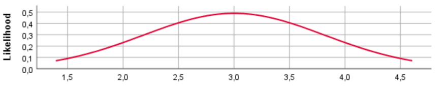
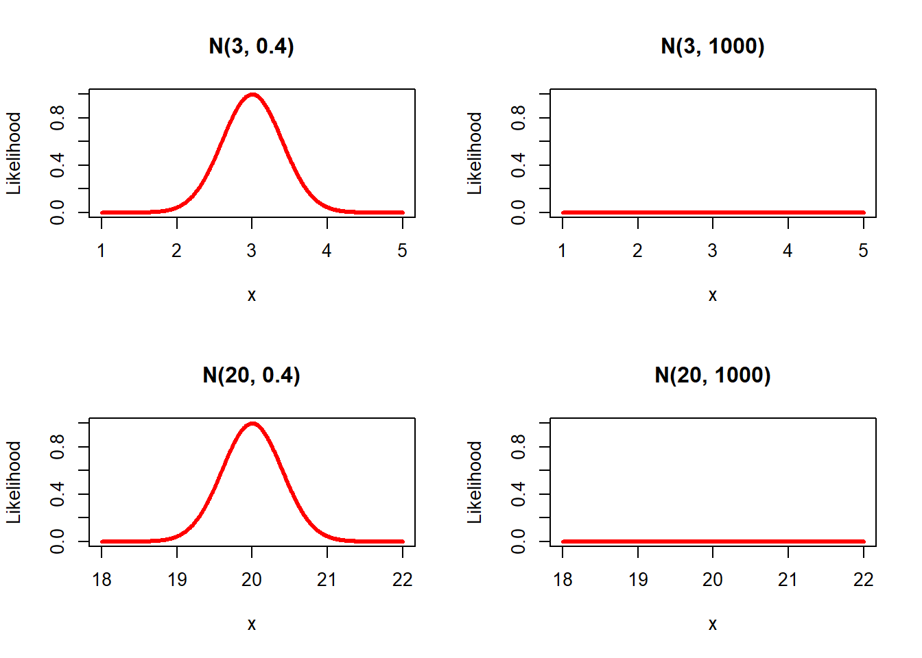
SPSS also provides plots of the prior, the likelihood and the posterior. Inspect the prior plots from SPSS.
SPSS plots
N(3, 0.4)
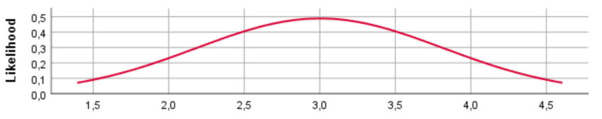
N(3, 1000)
N(20, 0.4)
N(20, 1000)
Default prior
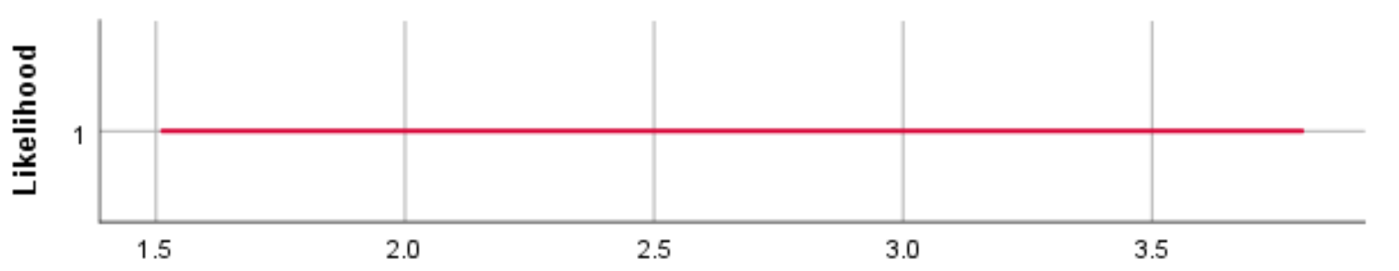
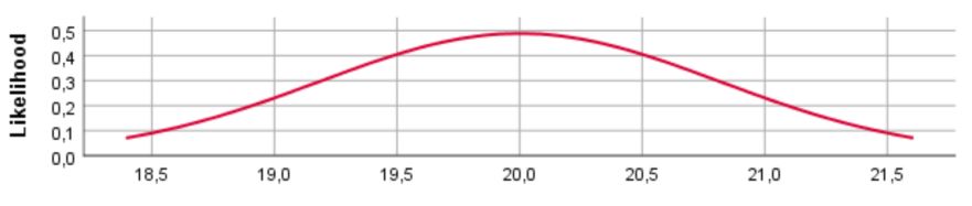
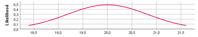
For the different prior distributions for the variable age we see a clear shift in the location of the distributions if the prior mean was changed. Regarding the variance, however, SPSS provides identical prior plots for different priors (At least when we ran the model). Probably this has been caused by a bug in SPSS. Below we show how the prior distributions really look like, by plotting them in R.
R plots
Question: Compare the results over the different prior specifications. Are the results comparable with the default model?
In these new plots we do not only see a shift in the mean, by changing the prior mean, but we also see the effect of the variance. That is, specifying a large variance such as 1000, results in a really flat prior.The results change a bit with different prior specifications, but are still comparable. Only using N(20, 0.4) for age, results in a somewhat different coefficient, since this prior mean is far from the mean of the data, while its variance is quite certain. However, in general the results are comparable. Because we use a big dataset the influence of the prior is relatively small. If one would use a smaller dataset the influence of the priors are larger. To check this you can use these lines to sample roughly 20% of all cases and redo the same analysis. The results will of course be different because we use many fewer cases (probably too few!). Use this code.
USE ALL.
COMPUTE filter_$=(uniform(1)<=.20).
VARIABLE LABELS filter_$ 'Approximately 20% of the cases (SAMPLE)'.
FORMATS filter_$ (f1.0).
FILTER  BY filter_$.
EXECUTE.Question: Do we end up with similar conclusions, using different prior specifications?
Finally, we end up with similar conclusions.
A logical next step is to define your own priors. To do so, one first needs to think about a plausible parameter space. You can follow the steps in this responsive tutorial to do so.
To study the impact of priors in more detail we recommend our Priors in SPSS exercise, and if you really want to use Bayes for your own data, we recommend to follow the WAMBS-checklist, which you are guided through by this exercise.