First Bayesian Inference: SPSS (T-test)
By Naomi Schalken, Lion Behrens, Laurent Smeets and Rens van de Schoot
Last modified: date: 03 november 2018
This tutorial provides the reader with a basic tutorial how to perform and interpret a Bayesian T-test in SPSS. Throughout this tutorial, the reader will be guided through importing datafiles, exploring summary statistics and conducting a T-test. Here, we will exclusively focus on Bayesian statistics. In this tutorial, we start by using the default prior settings of the software and then set some user-specified priors. If you really want to use Bayes for your own data, we recommend to follow the WAMBS-checklist, which you are guided through by this exercise.
Preparation
This Tutorial Expects:
- Basic knowledge of hypothesis testing
- Basic knowledge of Bayesian inference
- Any installed version of SPSS higher than 25 on your electronic device
Example Data
The data we will be using for this exercise is based on a study about predicting PhD-delays ( Van de Schoot, Yerkes, Mouw and Sonneveld 2013). The data can be downloaded here. Among many other questions, the researchers asked the Ph.D. recipients how long it took them to finish their Ph.D. thesis (n=333). It appeared that Ph.D. recipients took an average of 59.8 months (five years and four months) to complete their Ph.D. trajectory. The variable B3_difference_extra measures the difference between planned and actual project time in months (mean=9.96, minimum=-31, maximum=91, sd=14.43).
For the current exercise we would like to answer the question why some Ph.D. recipients took longer than others by investigating whether having had any children (up to the age 18) throughout the Ph.D. trajectory affects delays (0=No, 1=Yes). Out of the 333 respondents, 18% reported to have had at least one child.
So, in our model the PhD delays is the dependent variable and having a child is the predictor. The data can be found in the file phd-delays.csv .
Question: Write down the null and alternative hypothesis that represent this question.
H0: PhD recipients with and without children have similar PhD-delays.
H1: PhD recipients with and without children have different PhD-delays.
Preparation – Importing and Exploring Data
You can find the data in the file phd-delays.csv , which contains all variables that you need for this analysis. Although it is a .csv-file, you can directly load it into SPSS. If you do not know how, go to our How to Get Started With SPSS-exercise.
Once you loaded in your data, it is advisable to check whether your data import worked well. Therefore, first have a look at the summary statistics of your data (again, if you do not know how to obtain these estimates go to our How to Get Started With SPSS-exercise).
EXAMINE VARIABLES=B3_difference_extra E4_having_child
  /PLOT BOXPLOT STEMLEAF
  /COMPARE GROUPS
  /STATISTICS DESCRIPTIVES
  /CINTERVAL 95
  /MISSING LISTWISE
  /NOTOTAL.
Question: Have all your data been loaded in correctly? That is, do all data points substantively make sense? If you are unsure, go back to the .csv-file to inspect the raw data.
B3_difference_extra: Mean = 9.97, SE=0.791
E4_having_child: Mean= 0.18, SE=0.021
T-Test – Default Priors
In this exercise you will compare Ph.D. students who had children during their trajectory with those who hadn’t (0=No, 1=Yes) in the difference between their planned and actual project time in months_, _which serves as the outcome variable using an independent samples T-test.
As you know, Bayesian inference consists of combining a prior distribution with the likelihood obtained from the data. Specifying a prior distribution is one of the most crucial points in Bayesian inference and should be treated with your highest attention (for a quick refresher see e.g. Van de Schoot et al. 2014). In this tutorial, we will first rely on the default prior settings, thereby behaving a ‘naïve’ Bayesians (which might not always be a good idea).
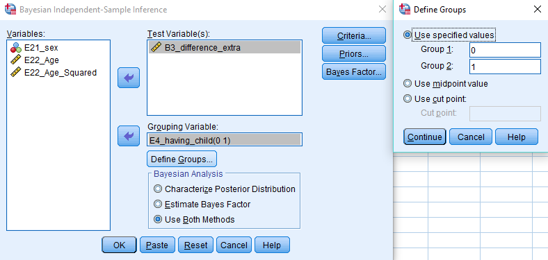
You can conduct your test by clicking Analyze -> Bayesian Statistics -> Independent Samples Normal and defining the values of the grouping variable E4_having_child. In the Bayesian Analysis tab, be sure to request both the posterior distribution and a Bayes factor by ticking Use Both Methods.
Alternatively, you can execute the following code in your syntax file:
BAYES INDEPENDENT
  /MISSING SCOPE=ANALYSIS
  /CRITERIA CILEVEL=95 TOL=0.000001 MAXITER=2000
  /INFERENCE DISTRIBUTION=NORMAL VARIABLES=B3_difference_extra ANALYSIS=BOTH GROUP=E4_having_child
    SELECT=LEVEL(0 1)
  /PRIOR EQUALDATAVAR=FALSE VARDIST=DIFFUSE
  /ESTBF COMPUTATION=ROUDER.
Question: Interpret the estimated effect and its interval using the posterior distribution.
The estimated mean difference between PhD recipients with and without children in their PhD project delays is 4.13, with a variance = 5.298, and a 95% Credibility Interval [-0.40, 8.65]. Because the credibility interval contains 0, it seems that having children or not is no relevant predictor for the PhD delays. There is a probability of 95% that the population value for the regression coefficient is within the limits of this interval.
In statistical inference, there is a fundamental difference between estimating a population parameter and testing hypotheses regarding it. So far, you gave estimation-based interpretations by characterizing the parameter’s posterior distribution. Now, you are going to test hypotheses with the Bayes factor, the counterpart of the frequentist p-value. Other than the p-value that tries to reject a null hypothesis, the Bayes factor directly compares the evidence for two (or more) hypotheses under consideration. Above, you formulated the null and alternative hypothesis for the research question under investigation. A Bayes factor compares the likelihood of population parameter values under all scenarios that are in line with the null hypothesis with their likelihood under all scenarios that are in line with the alternative hypothesis. Ultimately, it quantifies how much better the alternative hypothesis fits better than the null and vice versa. It thus directly compares two hypotheses and provides evidence for both, something that the p-value cannot do.
Question: Interpret the Bayes Factor.
The Bayes Factor = 1.275. This means there is relatively more evidence for the null hypothesis than for the alternative hypothesis. Although, the Bayes factor still doesn’t give strong support for one of both hypotheses. Please ignore the P-value in the Bayes Factor output.
Question: How does its interpretation differ from the classical p-value?
The difference with the classical p-value is that the Bayes Factor gives an indication of support for both hypotheses, and compares this evidence. Also, it says something about the strength of the evidence for the null hypothesis in comparison with the alternative hypothesis in this situation. On the other hand, the p-value is only able to support the decision of rejecting the null hypothesis or not.
Question: What are potential pitfalls to the interpretation of a Bayes Factor? After having collected your own ideas, have a look at Konijn et al. (2015) for further reasoning.
One of the main pitfalls of a Bayes factor, is that it could be used in the same way as a p-value, which is as a cut-off score. Of course, the Bayes factor indicates in which direction the evidence lies, but it isn’t supposed to be used in the same way as the p-value. It is therefore also possible, that a Bayes factor doesn’t give strong support for one of both hypotheses, like in the current exercise. Particularly in such situations, we should accept this result, and shouldn’t decide the null hypothesis is ‘true’, because a Bayes factor points somewhat more in that direction. The evidence is still not that strong.
T-test – User-specified Priors
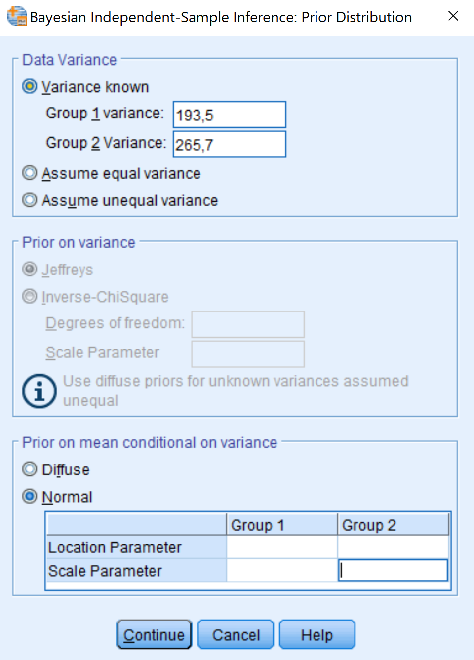
In SPSS, you can also manually specify your prior distributions. Be aware that usually, this has to be done BEFORE peeking at the data, otherwise you are double-dipping (!). In theory, you can specify your prior knowledge using any kind of distribution you like. However, in SPSS there are only a few options which can be adapted, dependent on the assumption of ‘equal group variances’. We won’t discuss this assumption in this exercise, but take the assumption that we have ‘known variances’ for the groups in this exercise. Based on this assumption, we can adapt the prior specifications for the group means, in the form of a normal distribution, by adapting the location and scale parameters. The location parameter indicates the mean of the group, and the scale parameter indicates the standard deviation of the group.
In SPSS we can specify the prior distributions for the groups ourselves, by going to Analyze -> Bayesian statistics -> Independent samples normal . Fill in the model like in the exercise above. Click on Priors , and then the menu in the picture below appears.
We assume that group variances are known. Hence, we say Group 1 has a variance of 193,5, and Group 2 has a variance of 265,7. Then we can specify normal prior distributions for Group 1 and 2. So first we have to provide a mean for Group 1 (location parameter) and a variance for Group 1 (Scale parameter). Followed by the mean and variance of Group 2. After we specified this, we can run the model.
In this example we use two variations of prior distributions, and compare this with the default results above.
First, we use this:
Group 1: Location (9), Scale (14)
Group 2: Location (13), Scale (16)
Second, we use:
Group 1: Location (20), Scale (5)
Group 2: Location (2), Scale (5)
The location parameter indicates the mean of the prior distribution and the scale parameter the width of this distribution.
Run both analyses, and report the results in the table below.
| B3_difference_extra | Default | First prior specification | Second prior specification |
|---|---|---|---|
| Posterior mean | |||
| Posterior variance |
Question: Compare the results with the ones using the default priors, are the results comparable?
Results:
| B3_difference_extra | Default | First prior specification | Second prior specification |
|---|---|---|---|
| Posterior mean | 4,13 | 4,28 | -2,62 |
| Posterior variance | 5,298 | 4,141 | 2,872 |
The results are not comparable over the different prior specifications. The first prior specification results in a posterior mean that is quite comparable with the default result. However, the second prior specification results in a complete different result.
Question: Do we end up with similar conclusions, using different prior specifications?
For the default and the first prior specifications, we end up with approximately similar results, that are in the same direction. However, for the second prior specification the result is the other way around. The reason for this, is that the first prior specification was really close to the results in the observed data. However, the second prior specification is not comparable at all with the observed data, and is in comparison to the first priors, more certain. This has the effect, that the prior influences the data as such, that it results in another conclusion. So according to results with default priors and the first prior specification, Group 2 (with children) has more delay than Group 1 (without children). Whereas, the analysis with the second prior specification, shows that Group 2 (with children) has less delay than Group 1 (without children).