Regression in lavaan (Frequentist)
By Laurent Smeets and Rens van de Schoot
Last modified: 19 October 2019
Introduction
This tutorial provides the reader with a basic tutorial how to perform a regression analysis in lavaan. Throughout this tutorial, the reader will be guided through importing datafiles, exploring summary statistics and regression analyses. Here, we will exclusively focus on frequentist statistics.
We are continuously improving the tutorials so let me know if you discover mistakes, or if you have additional resources I can refer to. The source code is available via Github. If you want to be the first to be informed about updates, follow me on Twitter.
Preparation
This tutorial expects:
- Installation of R package
lavaan. This tutorial was made using Lavaan version 0.6.5 in R version 3.6.1 - Basic knowledge of hypothesis testing
- Basic knowledge of correlation and regression
- Basic knowledge of coding in R
Example Data
The data we will be using for this exercise is based on a study about predicting PhD-delays (Van de Schoot, Yerkes, Mouw and Sonneveld 2013).The data can be downloaded here. Among many other questions, the researchers asked the Ph.D. recipients how long it took them to finish their Ph.D. thesis (n=333). It appeared that Ph.D. recipients took an average of 59.8 months (five years and four months) to complete their Ph.D. trajectory. The variable B3_difference_extra measures the difference between planned and actual project time in months (mean=9.97, minimum=-31, maximum=91, sd=14.43). For more information on the sample, instruments, methodology and research context we refer the interested reader to the paper.
For the current exercise we are interested in the question whether age (M = 31.7, SD = 6.86) of the Ph.D. recipients is related to a delay in their project.
The relation between completion time and age is expected to be non-linear. This might be due to that at a certain point in your life (i.e., mid thirties), family life takes up more of your time than when you are in your twenties or when you are older.
So, in our model the \(gap\) (B3_difference_extra) is the dependent variable and \(age\) (E22_Age) and \(age^2\)(E22_Age_Squared ) are the predictors. The data can be found in the file phd-delays.csv .
Question: Write down the null and alternative hypotheses that represent this question. Which hypothesis do you deem more likely?
< class="collapseomatic " id="id6863e5f077369"  tabindex="0" title=""    >
\(H_0:\) \(age\) is not related to a delay in the PhD projects.
\(H_1:\) \(age\) is related to a delay in the PhD projects.
\(H_0:\) \(age^2\) is not related to a delay in the PhD projects.
\(H_1:\) \(age^2\)is related to a delay in the PhD projects.
Preparation – Importing and Exploring Data
Install the following packages in R:
library(lavaan)
library(psych) #to get some extended summary statistics
library(tidyverse) # needed for data manipulation and plotting
You can find the data in the file phd-delays.csv , which contains all variables that you need for this analysis. Although it is a .csv-file, you can directly load it into R using the following syntax:
#read in data
dataPHD <- read.csv2(file="phd-delays.csv")
colnames(dataPHD) <- c("diff", "child", "sex","age","age2")
Alternatively, you can directly download them from GitHub into your R work space using the following command:
dataPHD <- read.csv2(file="https://raw.githubusercontent.com/LaurentSmeets/Tutorials/master/Blavaan/phd-delays.csv")
colnames(dataPHD) <- c("diff", "child", "sex","age","age2")
GitHub is a platform that allows researchers and developers to share code, software and research and to collaborate on projects (see https://github.com/)
Once you loaded in your data, it is advisable to check whether your data import worked well. Therefore, first have a look at the summary statistics of your data. you can do this by using the describe() function.
Question: Have all your data been loaded in correctly? That is, do all data points substantively make sense? If you are unsure, go back to the .csv-file to inspect the raw data.
describe(dataPHD)## vars n mean sd median trimmed mad min max range skew
## diff 1 333 9.97 14.43 5 6.91 7.41 -31 91 122 2.21
## child 2 333 0.18 0.38 0 0.10 0.00 0 1 1 1.66
## sex 3 333 0.52 0.50 1 0.52 0.00 0 1 1 -0.08
## age 4 333 31.68 6.86 30 30.39 2.97 26 80 54 4.45
## age2 5 333 1050.22 656.39 900 928.29 171.98 676 6400 5724 6.03
## kurtosis se
## diff 5.92 0.79
## child 0.75 0.02
## sex -2.00 0.03
## age 24.99 0.38
## age2 42.21 35.97The descriptive statistics make sense:
diff: Mean (9.97), SE (0.79)
\(Age\): Mean (31.68), SE (0.38)
\(Age^2\): Mean (1050.22), SE (35.97)
plot
Before we continue with analyzing the data we can also plot the expected relationship.
dataPHD %>%
  ggplot(aes(x = age,
             y = diff)) +
  geom_point(position = "jitter",
             alpha    = .6)+ #to add some random noise for plotting purposes
  theme_minimal()+
  geom_smooth(method = "lm",  # to add  the linear relationship
              aes(color = "linear"),
              se = FALSE) +
  geom_smooth(method = "lm",
              formula = y ~ x + I(x^2),# to add  the quadratic relationship
              aes(color = "quadratic"),
              se = FALSE) +
  labs(title    = "Delay vs. age",
       subtitle = "There seems to be some quadratic relationship",
       x        = "Age",
       y        = "Delay",
       color    = "Type of relationship" ) +
  theme(legend.position = "bottom")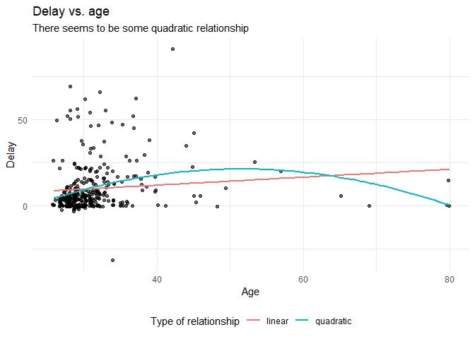
Regression Analysis
Now, let’s run a multiple regression model predicting the difference between Ph.D. students’ planned and actual project time by their age (note that we ignore assumption checking, if you want a quick introduction to the assumptions underlying a regression, please have look at https://statistics.laerd.com/spss-tutorials/linear-regression-using-spss-statistics.php).
To run a multiple regression with lavaan, you first specify the model, then fit the model and finally acquire the summary. The model is specified as follows:
- A depedent variable we want to predict.
- A “~”, that we use to indicate that we now give the other variables of interest. (comparable to the ‘=’ of the regression equation).
- The different indepedent variables separated by the summation symbol ‘+’.
- Finally, we specify that the dependent variable has a variance and that we want an intercept.
- To fit the model we use the
lavaan()function, which needs amodel=and adata=input.
For more information on the basics of lavaan, see their website
The following code is how to specify the regression model:
model.regression <- '#the regression model
                    diff ~ age + age2

                    #show that dependent variable has variance
                    diff ~~ diff

                    #we want to have an intercept
                    diff ~ 1'
Now, perform a multiple linear regression and answer the following question:
Question: Using a significance criterion of 0.05, is there a significant effect of \(age\) and \(age^2\)?
fit <- lavaan(model = model.regression, data = dataPHD)
summary(fit, fit.measures = TRUE, ci = TRUE, rsquare = TRUE)
## lavaan 0.6-5 ended normally after 24 iterations
##
## Estimator ML
## Optimization method NLMINB
## Number of free parameters 4
##
## Number of observations 333
##
## Model Test User Model:
##
## Test statistic 0.000
## Degrees of freedom 0
##
## Model Test Baseline Model:
##
## Test statistic 21.521
## Degrees of freedom 2
## P-value 0.000
##
## User Model versus Baseline Model:
##
## Comparative Fit Index (CFI) 1.000
## Tucker-Lewis Index (TLI) 1.000
##
## Loglikelihood and Information Criteria:
##
## Loglikelihood user model (H0) -1350.154
## Loglikelihood unrestricted model (H1) -1350.154
##
## Akaike (AIC) 2708.308
## Bayesian (BIC) 2723.541
## Sample-size adjusted Bayesian (BIC) 2710.852
##
## Root Mean Square Error of Approximation:
##
## RMSEA 0.000
## 90 Percent confidence interval - lower 0.000
## 90 Percent confidence interval - upper 0.000
## P-value RMSEA <= 0.05 NA
##
## Standardized Root Mean Square Residual:
##
## SRMR 0.000
##
## Parameter Estimates:
##
## Information Expected
## Information saturated (h1) model Structured
## Standard errors Standard
##
## Regressions:
## Estimate Std.Err z-value P(>|z|) ci.lower
## diff ~
## age 2.657 0.583 4.554 0.000 1.514
## age2 -0.026 0.006 -4.236 0.000 -0.038
## ci.upper
##
## 3.801
## -0.014
##
## Intercepts:
## Estimate Std.Err z-value P(>|z|) ci.lower
## .diff -47.088 12.285 -3.833 0.000 -71.166
## ci.upper
## -23.010
##
## Variances:
## Estimate Std.Err z-value P(>|z|) ci.lower
## .diff 194.641 15.084 12.903 0.000 165.076
## ci.upper
## 224.206
##
## R-Square:
## Estimate
## diff 0.063There is a significant effect of \(age\) and \(age^2\), with b=2.657, p <.001 for \(age\), and b=-0.026, p<.001 for \(age^2\).
Surveys in academia have shown that a large number of researchers interpret the p-value wrong and misinterpretations are way more widespread than thought. Have a look at the article by Greenland et al. (2016) that provides a guide to clear and concise interpretations of p.
Question: What can you conclude about the hypothesis being tested using the correct interpretation of the p-value?
Assuming that the null hypothesis is true in the population, the probability of obtaining a test statistic that is as extreme or more extreme as the one we observe is <0.1%. Because the effect of \(age^2\) is below our pre-determined alpha level, we reject the null hypothesis.
Recently, a group of 72 notable statisticians proposed to shift the significance threshold to 0.005 (Benjamin et al. 2017, but see also a critique byTrafimow, …, Van de Schoot, et al., 2018). They argue that a p-value just below 0.05 does not provide sufficient evidence for statistical inference.
Question: How does your conclusion change if you follow this advice?
Because the p-values for both regression coefficients were really small <.001, the conclusion doesn’t change in this case.
Of course, we should never base our decisions on single criterions only. Luckily, there are several additional measures that we can take into account. A very popular measure is the confidence interval. In the summary() function, these intervals can be demanded, which has already been done in the previous step.
Question: What can you conclude about the hypothesis being tested using the correct interpretation of the confidence interval?
\(Age\): 95% CI [1.514, 3.801]
\(Age^2\): 95% CI [-0.038, -0.014]
In both cases the 95% CI’s don’t contain 0, which means, the null hypotheses should be rejected. A 95% CI means, that, if infinitely samples were taken from the population, then 95% of the samples contain the true population value. But we do not know whether our current sample is part of this collection, so we only have an aggregated assurance that in the long run if our analysis would be repeated our sample CI contains the true population parameter.
Additionally, to make statements about the actual relevance of your results, focusing on effect size measures is inevitable.
Question: What can you say about the relevance of your results? Focus on the explained variance and the standardized regression coefficients.
R\(^2\)= 0.063 in the regression model. This means that 6.3% of the variance in the PhD delays, can be explained by \(age\) and \(age^2\).
We can also run the analysis again, but now with standardized coefficients.Lavaan has the inbuilt-function standardizedsolution() to obtain standardized coefficients.
standardizedsolution(fit)## lhs op rhs est.std se z pvalue ci.lower ci.upper
## 1 diff ~ age 1.262 0.265 4.763 0 0.743 1.782
## 2 diff ~ age2 -1.174 0.267 -4.402 0 -1.697 -0.651
## 3 diff ~~ diff 0.937 0.025 37.057 0 0.888 0.987
## 4 diff ~1 -3.268 0.819 -3.992 0 -4.872 -1.664
## 5 age ~~ age 1.000 0.000 NA NA 1.000 1.000
## 6 age ~~ age2 0.982 0.000 NA NA 0.982 0.982
## 7 age2 ~~ age2 1.000 0.000 NA NA 1.000 1.000
## 8 age ~1 4.627 0.000 NA NA 4.627 4.627
## 9 age2 ~1 1.602 0.000 NA NA 1.602 1.602The standardized coefficients, \(age\) (1.262) and \(age^2\) (-1.174), show that the effects of both regression coefficients are comparable, but the effect of \(age\) is somewhat higher.This means that the linear effect of age on PhD delay (age) is a bit larger than the quadratic effect of age on PhD delay (age2)
Only a combination of different measures assessing different aspects of your results can provide a comprehensive answer to your research question.
Question: Drawing on all the measures we discussed above, formulate an answer to your research question.
The variables \(age\) and \(age^2\) are significantly related to PhD delays. However, the total explained variance by those two predictors is only 6.3%. Therefore, a large part of the variance is still unexplained.
References
Benjamin, D. J., Berger, J., Johannesson, M., Nosek, B. A., Wagenmakers, E.,… Johnson, V. (2017, July 22). Redefine statistical significance. Retrieved from psyarxiv.com/mky9j
Greenland, S., Senn, S. J., Rothman, K. J., Carlin, J. B., Poole, C., Goodman, S. N. Altman, D. G. (2016). Statistical tests, P values, confidence intervals, and power: a guide to misinterpretations. European Journal of Epidemiology 31 (4). https://doi.org/10.1007/s10654-016-0149-3 _ _
_ Rosseel, Y. (2012)._ lavaan: An R Package for Structural Equation Modeling. Journal of Statistical Software, 48(2), 1-36.
van de Schoot R, Yerkes MA, Mouw JM, Sonneveld H (2013) What Took Them So Long? Explaining PhD Delays among Doctoral Candidates. PLoS ONE 8(7): e68839. https://doi.org/10.1371/journal.pone.0068839
Trafimow D, Amrhein V, Areshenkoff CN, Barrera-Causil C, Beh EJ, Bilgi? Y, Bono R, Bradley MT, Briggs WM, Cepeda-Freyre HA, Chaigneau SE, Ciocca DR, Carlos Correa J, Cousineau D, de Boer MR, Dhar SS, Dolgov I, G?mez-Benito J, Grendar M, Grice J, Guerrero-Gimenez ME, Guti?rrez A, Huedo-Medina TB, Jaffe K, Janyan A, Karimnezhad A, Korner-Nievergelt F, Kosugi K, Lachmair M, Ledesma R, Limongi R, Liuzza MT, Lombardo R, Marks M, Meinlschmidt G, Nalborczyk L, Nguyen HT, Ospina R, Perezgonzalez JD, Pfister R, Rahona JJ, Rodr?guez-Medina DA, Rom?o X, Ruiz-Fern?ndez S, Suarez I, Tegethoff M, Tejo M, ** van de Schoot R** , Vankov I, Velasco-Forero S, Wang T, Yamada Y, Zoppino FC, Marmolejo-Ramos F. (2017) Manipulating the alpha level cannot cure significance testing – comments on “Redefine statistical significance”_ _PeerJ reprints 5:e3411v1 https://doi.org/10.7287/peerj.preprints.3411v1