Regression in Mplus (Frequentist)
By Laurent Smeets and Rens van de Schoot
Last modified: 22 August 2019
Introduction
This tutorial provides the reader with a basic tutorial how to perform a regression analysis in Mplus. Throughout this tutorial, the reader will be guided through importing datafiles, exploring summary statistics and regression analyses. Here, we will exclusively focus on frequentist statistics.
We are continuously improving the tutorials so let me know if you discover mistakes, or if you have additional resources I can refer to. The source code is available via Github. If you want to be the first to be informed about updates, follow me on Twitter.
Preparation
This tutorial expects:
- any version of Mplus.This tutorial was made using Mplus version 8_3.
- Basic knowledge of hypothesis testing
- Basic knowledge of correlation and regression
- Basic knowledge of coding in Mplus
Example Data
The data we will be using for this exercise is based on a study about predicting PhD-delays (Van de Schoot, Yerkes, Mouw and Sonneveld 2013).The data can be downloaded here. Among many other questions, the researchers asked the Ph.D. recipients how long it took them to finish their Ph.D. thesis (n=333). It appeared that Ph.D. recipients took an average of 59.8 months (five years and four months) to complete their Ph.D. trajectory. The variable B3_difference_extra measures the difference between planned and actual project time in months (mean=9.97, minimum=-31, maximum=91, sd=14.43). For more information on the sample, instruments, methodology and research context we refer the interested reader to the paper.
For the current exercise we are interested in the question whether age (M = 31.7, SD = 6.86) of the Ph.D. recipients is related to a delay in their project.
The relation between completion time and age is expected to be non-linear. This might be due to that at a certain point in your life (i.e., mid thirties), family life takes up more of your time than when you are in your twenties or when you are older.
So, in our model the \(gap\) (B3_difference_extra) is the dependent variable and \(age\) (E22_Age) and \(age^2\)(E22_Age_Squared ) are the predictors. The data can be found in the file phd-delays_nonames.csv . (In Mplus the first row CANNOT have the variable names, these have already been deleted for you)
Question: Write down the null and alternative hypotheses that represent this question. Which hypothesis do you deem more likely?
\(H_0:\) \(age\) is not related to a delay in the PhD projects.
\(H_1:\) \(age\) is related to a delay in the PhD projects.
\(H_0:\) \(age^2\) is not related to a delay in the PhD projects.
\(H_1:\) \(age^2\)is related to a delay in the PhD projects.
Preparation – Importing and Exploring Data
You can find the data in the file phd-delays_nonames.csv , which contains all variables that you need for this analysis. Although it is a .csv-file, you can directly load it into Mplus using the following syntax:
TITLE: Mplus analysis summary
DATA: FILE IS phd-delays_nonames.csv;
VARIABLE: NAMES ARE diff child sex Age Age2;
USEVARIABLES ARE diff Age Age2;
OUTPUT: sampstat;
Once you loaded in your data, it is advisable to check whether your data import worked well. Therefore, first have a look at the summary statistics of your data. You can do this by looking at the sampstat ouput.
Question: Have all your data been loaded in correctly? That is, do all data points substantively make sense? If you are unsure, go back to the .csv-file to inspect the raw data.
MODEL RESULTS

                                                    Two-Tailed
                    Estimate       S.E.  Est./S.E.    P-Value

 Means
    DIFF               9.967      0.790     12.622      0.000
    AGE               31.676      0.375     84.433      0.000
    AGE2            1050.217     35.916     29.241      0.000
The descriptive statistics make sense:
\(diff\): Mean (9.97), SE (0.79)
\(Age\): Mean (31.68), SE (0.38)
\(Age^2\): Mean (1050.22), SE (35.92)
Plot
Before we continue with analyzing the data we can also plot the expected relationship. We can do this by adding the following code to the input syntax of Mplus and then in the top menu go to Plot > View plot > Scatterplots (sample value) > View > Set X to AGE > OK
PLOT:
TYPE IS PLOT1;
This gives us the following plot:
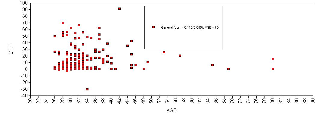
There seems to be some quadratic relationship
Regression Analysis
Now, let’s run a multiple regression model predicting the difference between Ph.D. students’ planned and actual project time by their age (note that we ignore assumption checking, if you want a quick introduction to the assumptions underlying a regression, please have look at https://statistics.laerd.com/spss-tutorials/linear-regression-using-spss-statistics.php).
To run a multiple regression with Mplus, you first specify the model, then fit the model and finally acquire the summary. The model is specified as follows:
- We set a title of the file under the
TITLE:command - We use a
DATAcommand and we tell Mplus what the datafile is called. - In the next syntax line, we use a
VARIABLEcommand that consists of two lines. First, we tell Mplus what the variable names are by using theNAMES AREstatement. Note that the order of the variable names has to mirror the actual order in the dataset. Second, we tell Mplus which variables we are actually going to use by usingUSEVARIABLES ARE. This way Mplus knows which columns in the.csvfile to use. - We specified a
MODELwhere an outcome variable (diff) is being regressedONtwo predictors (Age and Age2). Dependent or Y variables always appear on the left hand side of theONstatement and independent or X variables always appear on the right hand side of theONstatement. - We specify what types of output we would like after the
OUTPUTstatement. See here for a summary of all possible outputs and syntax
Now, preform a multiple linear regression and answer the following questions:
Question: Using a significance criterion of 0.05, is there a significant effect of \(age\) and \(age^2\)?
TITLE: Frequentist analysis

DATA: FILE IS phd-delays_nonames.csv;

VARIABLE: NAMES ARE diff child sex Age Age2; ! All the variables in the dataset

USEVARIABLES ARE diff Age Age2; ! The variables we use in this analysis

MODEL:
diff ON Age (Beta_Age);   ! Regression coefficient 1.
diff ON Age2(Beta_Age2);  ! Regression coefficient 2

OUTPUT: sampstat;
MODEL RESULTS
Two-Tailed
Estimate S.E. Est./S.E. P-Value
DIFF ON
AGE 2.657 0.583 4.554 0.000
AGE2 -0.026 0.006 -4.236 0.000
Intercepts
DIFF -47.088 12.285 -3.833 0.000
Residual Variances
DIFF 194.641 15.084 12.903 0.000There is a significant effect of \(age\) and \(age^2\), with b=2.657, p <.001 for \(age\), and b=-0.026, p<.001 for \(age^2\).
Surveys in academia have shown that a large number of researchers interpret the p-value wrong and misinterpretations are way more widespread than thought. Have a look at the article by Greenland et al. (2016) that provides a guide to clear and concise interpretations of p.
Question: What can you conclude about the hypothesis being tested using the correct interpretation of the p-value?
Assuming that the null hypothesis is true in the population, the probability of obtaining a test statistic that is as extreme or more extreme as the one we observe is <0.1%. Because the effect of \(age^2\) is below our pre-determined alpha level, we reject the null hypothesis.
Recently, a group of 72 notable statisticians proposed to shift the significance threshold to 0.005 (Benjamin et al. 2017, but see also a critique byTrafimow, …, Van de Schoot, et al., 2018). They argue that a p-value just below 0.05 does not provide sufficient evidence for statistical inference.
Question: How does your conclusion change if you follow this advice?
Because the p-values for both regression coefficients were really small <.001, the conclusion doesn’t change in this case.
Of course, we should never base our decisions on single criterions only. Luckily, there are several additional measures that we can take into account. A very popular measure is the confidence interval. To get the confidence intervals for the model parameters, you can add CINTERVAL to the OUTPUT statement in the input file, like
OUTPUT: sampstat CINTERVAL;This will give this output:
CONFIDENCE INTERVALS OF MODEL RESULTS

                  Lower .5%  Lower 2.5%    Lower 5%    Estimate    Upper 5%  Upper 2.5%   Upper .5%

 DIFF     ON
    AGE              1.154       1.514       1.697       2.657       3.617       3.801       4.160
    AGE2            -0.042      -0.038      -0.036      -0.026      -0.016      -0.014      -0.010

 Intercepts
    DIFF           -78.732     -71.167     -67.297     -47.088     -26.880     -23.010     -15.445

 Residual Variances
    DIFF           155.787     165.076     169.827     194.641     219.455     224.207     233.496
Question: What can you conclude about the hypothesis being tested using the correct interpretation of the confidence interval?
\(Age\): 95% CI [1.514, 3.801]
\(Age^2\): 95% CI [-0.038, -0.014]
In both cases the 95% CI’s don’t contain 0, which means, the null hypotheses should be rejected. A 95% CI means, that, if infinitely samples were taken from the population, then 95% of the samples contain the true population value. But we do not know whether our current sample is part of this collection, so we only have an aggregated assurance that in the long run if our analysis would be repeated our sample CI contains the true population parameter.
Additionally, to make statements about the actual relevance of your results, focusing on effect size measures is inevitable.
Question: What can you say about the relevance of your results? Focus on the explained variance and the standardized regression coefficients.
To get the standardized results and an estimate of the explained variance (R\(^2\)), you can add CINTERVAL to the OUTPUT statement in the input file, like
OUTPUT: sampstat CINTERVAL STDYX;R-SQUARE
Observed Two-Tailed
Variable Estimate S.E. Est./S.E. P-Value
DIFF 0.063 0.026 2.435 0.015R\(^2\)= 0.063 in the regression model. This means that 6.3% of the variance in the PhD delays, can be explained by \(age\) and \(age^2\).
STDYX Standardization

                                                    Two-Tailed
                    Estimate       S.E.  Est./S.E.    P-Value

 DIFF     ON
    AGE                1.262      0.269      4.685      0.000
    AGE2              -1.174      0.271     -4.340      0.000

 Intercepts
    DIFF              -3.268      0.819     -3.992      0.000

 Residual Variances
    DIFF               0.937      0.026     36.472      0.000
The standardized coefficients, age (1.262) and age\(^2\) (-1.174), show that the effects of both regression coefficients are comparable, but the effect of age is somewhat higher. This means that the linear effect of age on PhD delay (age) is a bit larger than the quadratic effect of age on PhD delay (age2)
Only a combination of different measures assessing different aspects of your results can provide a comprehensive answer to your research question.
Question: Drawing on all the measures we discussed above, formulate an answer to your research question.
The variables \(age\) and \(age^2\) are significantly related to PhD delays. However, the total explained variance by those two predictors is only 6.3%. Therefore, a large part of the variance is still unexplained.
References
Benjamin, D. J., Berger, J., Johannesson, M., Nosek, B. A., Wagenmakers, E.,… Johnson, V. (2017, July 22). Redefine statistical significance. Retrieved from psyarxiv.com/mky9j
Greenland, S., Senn, S. J., Rothman, K. J., Carlin, J. B., Poole, C., Goodman, S. N. Altman, D. G. (2016). Statistical tests, P values, confidence intervals, and power: a guide to misinterpretations. European Journal of Epidemiology 31 (4). https://doi.org/10.1007/s10654-016-0149-3 _ _
van de Schoot R, Yerkes MA, Mouw JM, Sonneveld H (2013) What Took Them So Long? Explaining PhD Delays among Doctoral Candidates. PLoS ONE 8(7): e68839. https://doi.org/10.1371/journal.pone.0068839
Trafimow D, Amrhein V, Areshenkoff CN, Barrera-Causil C, Beh EJ, Bilgi? Y, Bono R, Bradley MT, Briggs WM, Cepeda-Freyre HA, Chaigneau SE, Ciocca DR, Carlos Correa J, Cousineau D, de Boer MR, Dhar SS, Dolgov I, G?mez-Benito J, Grendar M, Grice J, Guerrero-Gimenez ME, Guti?rrez A, Huedo-Medina TB, Jaffe K, Janyan A, Karimnezhad A, Korner-Nievergelt F, Kosugi K, Lachmair M, Ledesma R, Limongi R, Liuzza MT, Lombardo R, Marks M, Meinlschmidt G, Nalborczyk L, Nguyen HT, Ospina R, Perezgonzalez JD, Pfister R, Rahona JJ, Rodr?guez-Medina DA, Rom?o X, Ruiz-Fern?ndez S, Suarez I, Tegethoff M, Tejo M, ** van de Schoot R** , Vankov I, Velasco-Forero S, Wang T, Yamada Y, Zoppino FC, Marmolejo-Ramos F. (2017) Manipulating the alpha level cannot cure significance testing – comments on “Redefine statistical significance”_ _PeerJ reprints 5:e3411v1 https://doi.org/10.7287/peerj.preprints.3411v1