Preparation

This Tutorial Expects:

• Basic knowledge of correlation and regression
• Any installed version higher than 24 on your electronic device

Example Data

The data we will be using for this exercise is based on a study about predicting PhD-delays (Van de Schoot, Yerkes, Mouw and Sonneveld 2013).The data can be downloaded here. Among many other questions, the researchers asked the Ph.D. recipients how long it took them to finish their Ph.D. thesis (n=333). It appeared that Ph.D. recipients took an average of 59.8 months (five years and four months) to complete their Ph.D. trajectory. The variable B3_difference_extra measures the difference between planned and actual project time in months (mean=9.96, minimum=-31, maximum=91, sd=14.43). For more information on the sample, instruments, methodology and research context we refer the interested reader to the paper.

For the current exercise we are interested in the question whether age of the Ph.D. recipients is related to a delay in their project.

The relation between completion time and age is expected to be non-linear. This might be due to the fact that at a certain point in your life priorities shift (i.e., in your mid thirties family life takes up more of your time than when you are younger or older).

So, in our model the GAP is the dependent variable and AGE and AGE2 are the predictors. The data can be found in the file phd-delays.csv.

Question: Write down the null and alternative hypothesis that represent this question.

Preparation – Importing and Exploring Data

You can find the data in the file phd-delays.csv, which contains all variables that you need for this analysis. Although it is a .csv-file, you can directly load it into SPSS using the following syntax:

/GET DATA  /TYPE=TXT 
/FILE="C: your working directory\phd-delays.csv"  
/ENCODING='UTF8'  
/DELCASE=LINE  
/DELIMITERS=";"  
/ARRANGEMENT=DELIMITED  
/FIRSTCASE=2  
/IMPORTCASE=ALL  
/VARIABLES=  
B3_difference_extra F2.0  
E4_having_child F1.0  
E21_sex F1.0  
E22_Age F2.0.  
CACHE.  
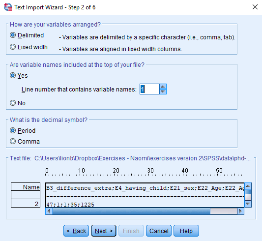
EXECUTE

Be aware that you need to specify your own working directory in the third line of the code. Alternatively, you can read the data in through the user interface, by clicking File -> Open -> Data and choosing phd-delays.csv. A window will pop up as shown below. Be sure to tick that the dataset’s first line consists of the variable names.

Once you loaded in your data, it is advisable to check whether your data import worked well. Therefore, first have a look at the summary statistics of your data. You can do so by clicking Analyze -> Descriptive Statistics -> Descriptives. Alternatively, to construct a reproducible analysis, you can open a new syntax file by clicking File -> New -> Syntax and executing the following syntax:

DESCRIPTIVES
VARIABLES=B3_difference_extra E22_Age E22_Age_Squared
/STATISTICS=MEAN SUM STDDEV VARIANCE RANGE MIN MAX SEMEAN. 

Question: Have all your data been loaded in correctly? That is, do all data points substantively make sense? If you are unsure, go back to the .csv-file to inspect the raw data.

Regression Analysis

Now, let’s run a multiple regression model predicting the difference between Ph.D. students’ planned and actual project time by their age (note that we ignore assumption checking, if you want a quick introduction to the assumptions underlying a regression, please have look at https://statistics.laerd.com/spss-tutorials/linear-regression-using-spss-statistics.php). Via the point-and-click method: Analyze -> Regression -> Linear

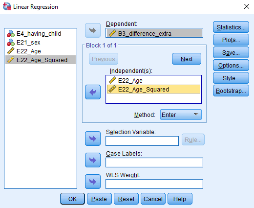
Alternatively, you can execute the following code in your syntax file:

REGRESSION
/MISSING PAIRWISE
/STATISTICS COEFF OUTS CI(95) R ANOVA
/CRITERIA=PIN(.05) POUT(.10)
/NOORIGIN
/DEPENDENT B3_difference_extra
/METHOD=ENTER E22_Age E22_Age_Squared.

Perform a multiple linear regression and answer the following questions:

Question: Using a significance criterion of 0.05, is there a significant effect of age and age2?

Surveys in academia have shown that a large number of researchers interpret the p-value wrong and misinterpretations are way more widespread than thought. Have a look at the article by Greenland et al. (2016) that provides a guide to clear and concise interpretations of p. _ _

Question: What can you conclude about the hypothesis being tested using the correct interpretation of the p-value?

Recently, a group of 72 notable statisticians proposed to shift the significance threshold to 0.005 ( Benjamin et al. 2017, but see also a critique by Trafimow, ., Van de Schoot, et al., 2018). They argue that a p-value just below 0.05 does not provide sufficient evidence for statistical inference.

Question: How does your conclusion change if you follow this advice?

Of course, we should never base our decisions on single criterions only. Luckily, there are several additional measures that we can take into account. A very popular measure is the confidence interval.

Question: What can you conclude about the hypothesis being tested using the correct interpretation of the confidence interval?

Additionally, to make statements about the actual relevance of your results, focusing on effect size measures is inevitable.

Question: What can you say about the relevance of your results? Focus on the explained variance and the standardized regression coefficients.

Only a combination of different measures assessing different aspects of your results can provide a comprehensive answer to your research question.

Question: Drawing on all the measures we discussed above, formulate an answer to your research question.

References

Benjamin, D. J., Berger, J., Johannesson, M., Nosek, B. A., Wagenmakers, E.,… Johnson, V. (2017, July 22). Redefine statistical significance. Retrieved from psyarxiv.com/mky9j

Greenland, S., Senn, S. J., Rothman, K. J., Carlin, J. B., Poole, C., Goodman, S. N. Altman, D. G. (2016). Statistical tests, P values, confidence intervals, and power: a guide to misinterpretations. European Journal of Epidemiology 31 (4). https://doi.org/10.1007/s10654-016-0149-3 _ _

van de Schoot R, Yerkes MA, Mouw JM, Sonneveld H (2013) What Took Them So Long? Explaining PhD Delays among Doctoral Candidates. PLoS ONE 8(7): e68839. https://doi.org/10.1371/journal.pone.0068839

Trafimow D, Amrhein V, Areshenkoff CN, Barrera-Causil C, Beh EJ, Bilgiç Y, Bono R, Bradley MT, Briggs WM, Cepeda-Freyre HA, Chaigneau SE, Ciocca DR, Carlos Correa J, Cousineau D, de Boer MR, Dhar SS, Dolgov I, Gómez-Benito J, Grendar M, Grice J, Guerrero-Gimenez ME, Gutiérrez A, Huedo-Medina TB, Jaffe K, Janyan A, Karimnezhad A, Korner-Nievergelt F, Kosugi K, Lachmair M, Ledesma R, Limongi R, Liuzza MT, Lombardo R, Marks M, Meinlschmidt G, Nalborczyk L, Nguyen HT, Ospina R, Perezgonzalez JD, Pfister R, Rahona JJ, Rodríguez-Medina DA, Romão X, Ruiz-Fernández S, Suarez I, Tegethoff M, Tejo M, ** van de Schoot R** , Vankov I, Velasco-Forero S, Wang T, Yamada Y, Zoppino FC, Marmolejo-Ramos F. (2017) Manipulating the alpha level cannot cure significance testing – comments on “Redefine statistical significance”_ _PeerJ reprints 5:e3411v1 https://doi.org/10.7287/peerj.preprints.3411v1