T-test in SPSS (Frequentist)
By Naomi Schalken, Lion Behrens, Laurent Smeets and Rens van de Schoot
Last modified: date: 29 oktober 2018
Developed for SPSS version 24 or 25
This tutorial provides the reader with a basic tutorial how to perform and interpret a T-test in SPSS. Throughout this tutorial, the reader will be guided through importing datafiles, exploring summary statistics and conducting a T-test. Here, we will exclusively focus on frequentist statistics.
To conduct the same analysis using Bayesian statistics, click here for your Bayes tutorial!
Preparation
This Tutorial Expects:
- Basic knowledge of T-tests
- Any installed version of SPSS. Note, the syntax and the tables presented in this tutorial make use of the SPSS version 25 interface.
Example Data
The data we will be using for this exercise is based on a study about predicting PhD-delays ( Van de Schoot, Yerkes, Mouw and Sonneveld 2013). The data can be downloaded here. Among many other questions, the researchers asked the Ph.D. recipients how long it took them to finish their Ph.D. thesis (n=333). It appeared that Ph.D. recipients took an average of 59.8 months (five years and four months) to complete their Ph.D. trajectory. The variable B3_difference_extra measures the difference between planned and actual project time in months (mean=9.96, minimum=-31, maximum=91, sd=14.43).
For the current exercise we would like to answer the question why some Ph.D. recipients took longer than others by investigating whether having had any children (up to the age 18) throughout the Ph.D. trajectory affects delays (0=No, 1=Yes). Out of the 333 respondents, 18% reported to have had at least one child.
So, in our model the PhD delays is the dependent variable and having a child is the predictor. The data can be found in the file phd-delays.csv .
Question: Write down the null and alternative hypothesis that represent this question.
H0: PhD recipients with and without children have similar PhD-delays.
H1: PhD recipients with and without children have different PhD-delays.
Preparation – Importing and Exploring Data
You can find the data in the file phd-delays.csv , which contains all variables that you need for this analysis. Although it is a .csv-file, you can directly load it into SPSS using the following syntax:
/GET DATA /TYPE=TXT
/FILE="C: your working directory\phd-delays.csv"
/ENCODING='UTF8'
/DELCASE=LINE
/DELIMITERS=";"
/ARRANGEMENT=DELIMITED
/FIRSTCASE=2
/IMPORTCASE=ALL
/VARIABLES=
B3_difference_extra F2.0
E4_having_child F1.0
E21_sex F1.0
E22_Age F2.0
E22_Age_Squared F2.0.
CACHE.
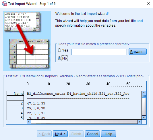
EXECUTE. Be aware that you need to specify your own working directory in the third line of the code. Alternatively, you can read the data in through the user interface, by clicking File -> Open -> Data and choosing phd-delays.csv. A window will pop up as shown below. Be sure to tick that the dataset’s first line consists of the variable names.
Once you loaded in your data, it is advisable to check whether your data import worked well. Therefore, first have a look at the summary statistics of your data. You can do so by clicking Analyze -> Descriptive Statistics -> Descriptives . Alternatively, to construct a reproducible analysis, you can open a new syntax file by clicking File -> New -> Syntax and executing the following syntax:
EXAMINE VARIABLES=B3_difference_extra E4_having_child
  /PLOT BOXPLOT STEMLEAF
  /COMPARE GROUPS
  /STATISTICS DESCRIPTIVES
  /CINTERVAL 95
  /MISSING LISTWISE
  /NOTOTAL.

or

DESCRIPTIVES
VARIABLES=B3_difference_extra E4_having_child
/STATISTICS=MEAN SUM STDDEV VARIANCE RANGE MIN MAX SEMEAN.
Question: Have all your data been loaded in correctly? That is, do all data points substantively make sense? If you are unsure, go back to the .csv-file to inspect the raw data.
The descriptive statistics make sense:
B3_difference_extra: Mean = 9.97, SE=0.791
E4_having_child: Mean= 0.18 (=18%), SE=0.021
T-Test
In this exercise you will compare Ph.D. students who had children during their trajectory with those who hadn’t (0=No, 1=Yes) in the difference between their planned and actual project time in months_, _which serves as the outcome variable using an independent samples T-test (note that we ignore assumption checking!). You can conduct your test by clicking Analyze -> Compare Means-> Independent Samples T-Test and defining the values of the grouping variable E4_having_child.

Alternatively, you can execute the following code in your syntax file:
T-TEST GROUPS= E4_having_child (0 1)
 /MISSING=ANALYSIS
 /VARIABLES=B3_difference_extra
 /CRITERIA=CI(.95).
Perform an independent samples t-test and interpret the output.
Question: Using a significance criterion of 0.05, is there a significant effect?
The result can be found in the ‘Independent Samples Test’ table. However, before we can inspect the results, we should have a look at Levene’s test of homogeneity of variances. Because Levene’s test is significant, F=4.517, p=0.034, we should look at the second row for the results. Based on these results, we are not able to reject H0, and therefore conclude that PhD recipients with and without children are not significantly different in their PhD delays, with t(78.96)=-1.821, p=.072.
Surveys in academia have shown that a large number of researchers interpret the p-value wrong and misinterpretations are way more widespread than thought. Have a look at the article by Greenland et al. (2016) that provides a guide to clear and concise interpretations of p.
Question: What can you conclude about the hypothesis being tested using the correct interpretation of the p-value?
Assuming that the null hypothesis is true in the population, the probability of obtaining a test statistic that is as extreme or more extreme as the one we observe is 7.2%. Because the effect is above our pre-determined alpha level we fail to reject the null hypothesis.
Recently, a group of 72 notable statisticians proposed to shift the significance threshold to 0.005 ( Benjamin et al. 2017, but see also a critique by Trafimow, ., Van de Schoot, et al., 2018 ). They argue that a p-value just below 0.05 does not provide sufficient evidence for statistical inference.
Question: How does your conclusion change if you follow this advice?
The conclusion doesn’t change here, but it becomes more obvious that the null hypothesis shouldn’t be rejected.
Of course, we should never base our decisions on single criterions only. Luckily, there are several additional measures that we can take into account. A very popular measure is the confidence interval.
Question: What can you conclude about the hypothesis being tested using the correct interpretation of the confidence interval?
The 95% CI [-8.638, 0.385].
The 95% CI’s does contain 0, which means, the null hypotheses should not be rejected. A 95% CI means, that if infinitely samples were taken from the population, then 95% of the samples contain the true population value. But we do not know whether our current sample is part of this collection, so we only have an aggregated assurance that in the long run if our analysis would be repeated our sample CI contains the true population parameter.
Additionally, to make statements about the actual relevance of your results, focusing on effect size measures is inevitable.
Question: What can you say about the relevance of your results? Focus on the mean difference between the groups and calculate Cohen’s D. If you are unsure how to calculate it, consult Cohen (1992).
Cohen’s d can be calculated as follows:
\[\hat{d}=\frac{\bar{X_1} – \bar{X_2}}{s}=\frac{9.22 – 13.35}{s_p}=\frac{9.22 – 13.35}{14.365}= -0.2875\]
Because the SD’s are not equal for both groups, we should calculate a pooled SD:
\[s_p = \sqrt\frac{(N_1 -1)s^{2}_{1} + (N_2 -1)s^{2}_{2}}{N_1 + N-_2 -2}=\sqrt\frac{(273 -1)13.910^{2} + (60 -1)16.300^{2}}{273 + 60 -2}=14.365\]
According to Cohen’s definitions, this is a small to medium effect.
d = 0.2 (small)
d = 0.5 (medium)
d = 0.8 (large)
Only a combination of different measures assessing different aspects of your results can provide a comprehensive answer to your research question.
Question: Drawing on all the measures we discussed above, formulate an answer to your research question.
Based on the above measures, we cannot reject the null hypothesis, because p = .072 and 95% CI [-8.638, 0.385]. However, we also couldn’t say the null hypothesis is ‘true’, or the difference between the groups is equal to 0. Besides that, Cohen’s d indicates there is a small to medium effect. Therefore, it becomes clear that making a decision only based on a p-value is not sufficient, and other measures should be considered as well.
References
Benjamin, D. J., Berger, J., Johannesson, M., Nosek, B. A., Wagenmakers, E.,… Johnson, V. (2017, July 22). Redefine statistical significance. Retrieved from psyarxiv.com/mky9j
Greenland, S., Senn, S. J., Rothman, K. J., Carlin, J. B., Poole, C., Goodman, S. N. Altman, D. G. (2016). Statistical tests, P values, confidence intervals, and power: a guide to misinterpretations. European Journal of Epidemiology 31 (4). https://doi.org/10.1007/s10654-016-0149-3
van de Schoot R, Yerkes MA, Mouw JM, Sonneveld H (2013) What Took Them So Long? Explaining PhD Delays among Doctoral Candidates. PLoS ONE 8(7): e68839. https://doi.org/10.1371/journal.pone.0068839
Trafimow D, Amrhein V, Areshenkoff CN, Barrera-Causil C, Beh EJ, Bilgiç Y, Bono R, Bradley MT, Briggs WM, Cepeda-Freyre HA, Chaigneau SE, Ciocca DR, Carlos Correa J, Cousineau D, de Boer MR, Dhar SS, Dolgov I, Gómez-Benito J, Grendar M, Grice J, Guerrero-Gimenez ME, Gutiérrez A, Huedo-Medina TB, Jaffe K, Janyan A, Karimnezhad A, Korner-Nievergelt F, Kosugi K, Lachmair M, Ledesma R, Limongi R, Liuzza MT, Lombardo R, Marks M, Meinlschmidt G, Nalborczyk L, Nguyen HT, Ospina R, Perezgonzalez JD, Pfister R, Rahona JJ, Rodríguez-Medina DA, Romão X, Ruiz-Fernández S, Suarez I, Tegethoff M, Tejo M, …, van de Schoot R, Vankov I, Velasco-Forero S, Wang T, Yamada Y, Zoppino FC, Marmolejo-Ramos F. (2017) Manipulating the alpha level cannot cure significance testing – comments on “Redefine statistical significance” PeerJ reprints 5:e3411v1 https://doi.org/10.7287/peerj.preprints.3411v1